Modelling the performance of a stormwater treatment train in a residential subdivision

Table of Contents

1. Introduction
2. Site Description
3. Approach/Methodology
4. Findings
5. Conclusions and Recommendations
6. References
7. Appendix A: Monitoring Approach
8. Appendix B: Model Set-up Details and Parameters

Introduction

This report presents the outcomes of a calibrated stormwater management model (SWMM) that represents a residential subdivision with a low impact development treatment train and a downstream stormwater management wet pond. It includes a discussion of essential parameters and methods for stormwater modelling in future designs.

This model was developed using Stormwater Management Model (EPA SWMM) software, which is freely available through the United States Environmental Protection Agency website.

Intensive hydrology monitoring has been conducted by Credit Valley Conservation’s Stormwater Science and Guidance (SSG) program from April 2015 to October 2018. Monitoring data shows that the stormwater management pond does not stabilize at the expected permanent pool level, but instead varies seasonally with the lowest levels observed in the summer and fall. By contrast, during the winter and spring, the pond will stabilize at or above the permanent pool level, resulting in the pond often flowing continuously. These monitoring outcomes were published in the report titled Stormwater Management Performance Summary: Meadows in the Glen Residential Subdivision (Credit Valley Conservation, 2021).

This technical brief uses a calibrated stormwater model based on robust on-site monitoring data to gain a better understanding of the stormwater management treatment train design and performance including:

• Question 1: What insights can we gain from the modelling exercise regarding the original design and its modelling process?
• Question 2: What are the drivers of the seasonal pattern observed in the stormwater management pond?
• Question 3: What are some challenges and lessons learned for modelling a site with a treatment train stormwater management approach?

Site Description

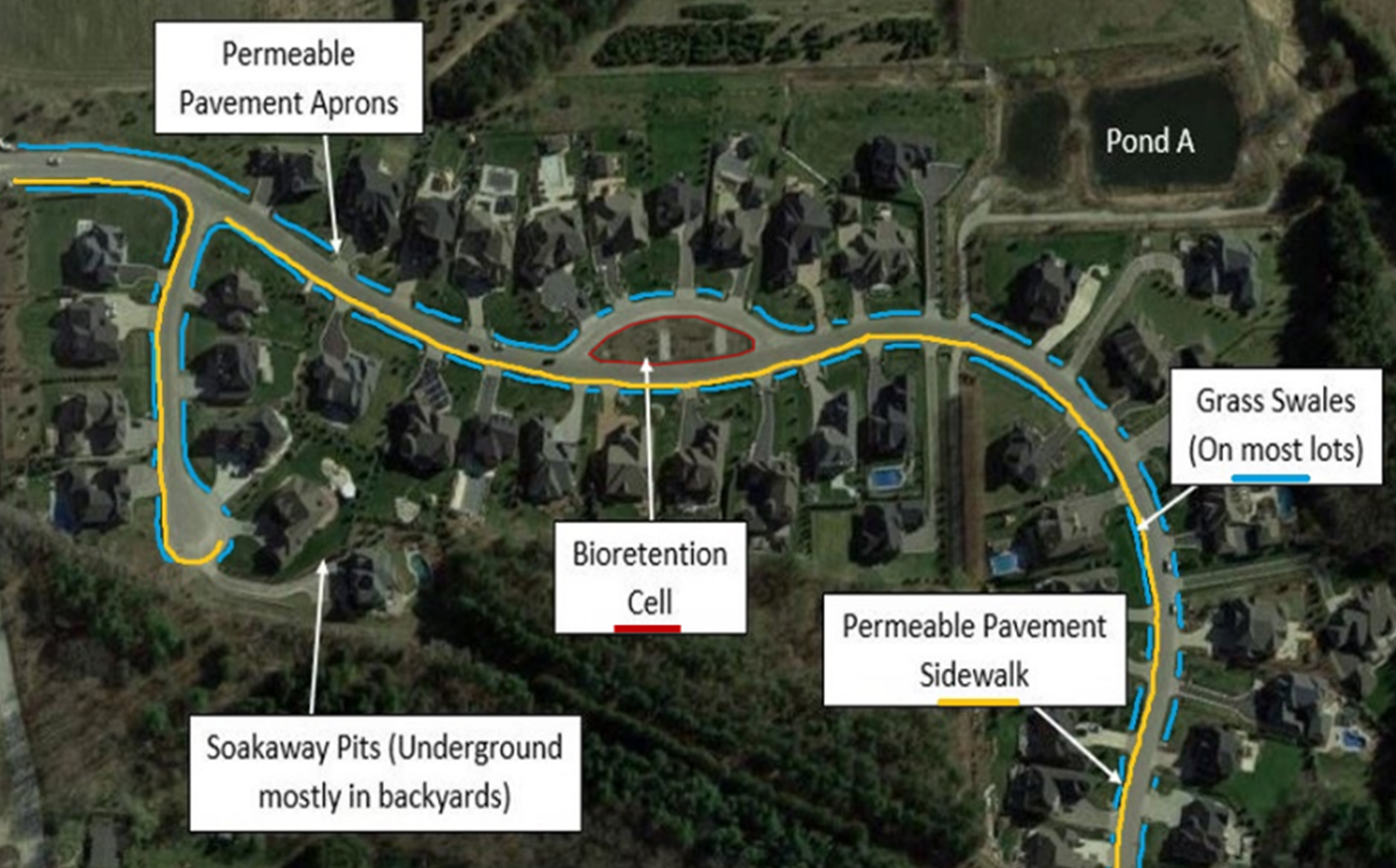
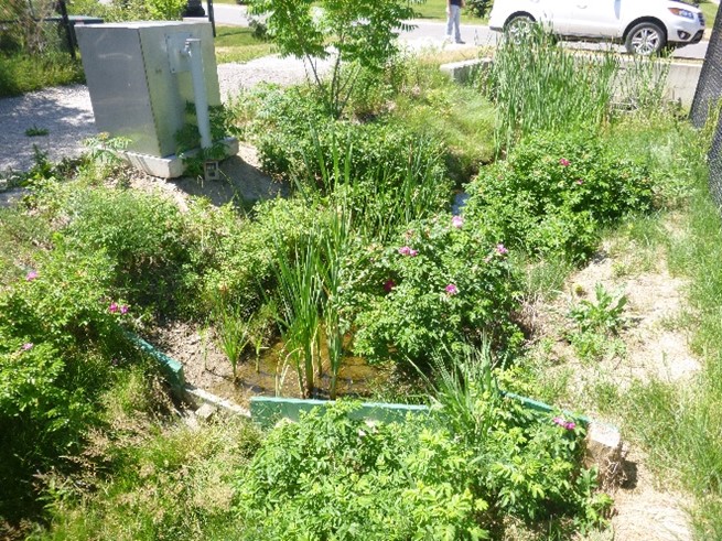
Meadows in the Glen (MITG) is the first subdivision in Halton Hills designed to manage stormwater using low impact development (LID) principles along with traditional stormwater management practices. MITG is a 27.5 hectare low density residential development with 35 per cent impervious cover.

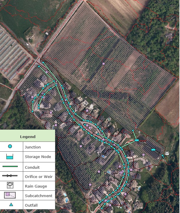
Imperviousness was reduced by using pervious pavement for sidewalks and driveway aprons, substituting sewers with grass swales, using native plantings, and retaining existing woodlots. Most properties have soakaway pits to infiltrate roof runoff, and a bioretention cell retains a portion of some of the road runoff. The subdivision consists of 91 lots and includes single-family homes, roads, parks, open space blocks, and two wet pond facilities (Pond A and Pond B) (Stantec, 2007a). This study will specifically focus on the catchment of Pond A, which is shown in Figure 1.

The subdivision is on lands previously owned by Sheridan Nurseries. Construction began in 2010 and continued through to 2014. Prior to development, the site was under active agricultural land use comprising non-native nursery stock, several plantations, a small woodlot, and some small patches of woodland and wetland. Sheridan Nurseries continue to cultivate commercial nursery stock on the neighbouring property. Under post-development conditions the eastern catchment, which includes 9.2 hectares of the MITG subdivision and 15.3 hectares from the adjacent Sheridan Nursery property, drains to the stormwater management facility (Pond A). Pond A is approximately 0.77 hectares and outlets to Tributary F. For additional site description and design criteria, refer to (Credit Valley Conservation, 2021).

Approach/Methodology

Monitoring

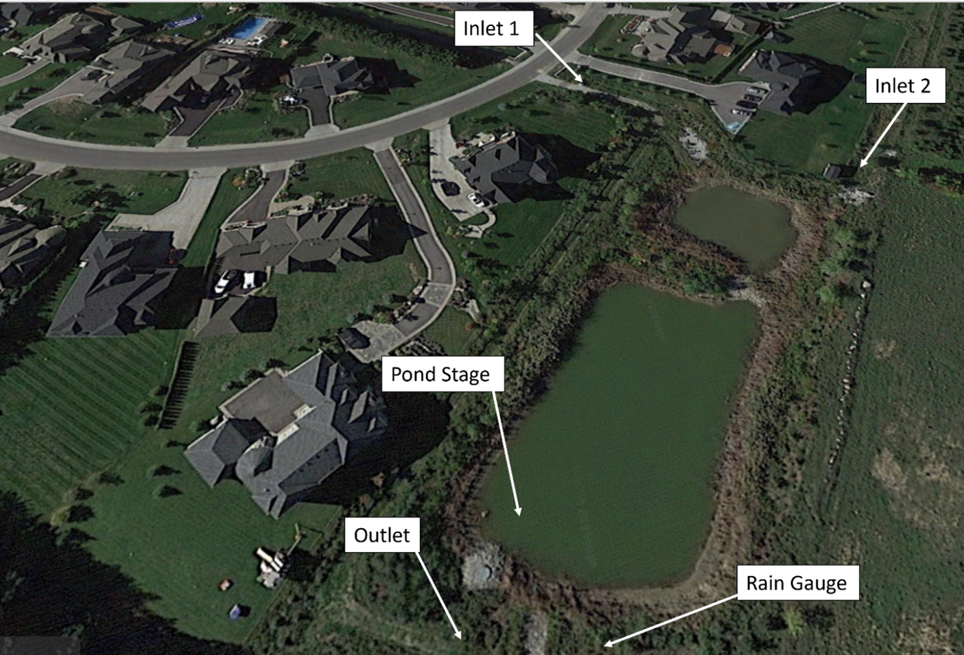
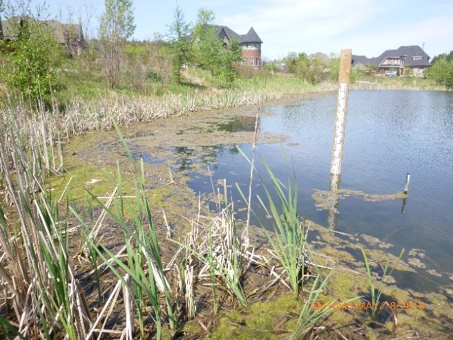
Monitoring was conducted at four stations located around Pond A: Inlet 1, Inlet 2, Outlet and Pond A Stage (Figure 2). Monitoring was also conducted at Tributary F, in groundwater wells around the subdivision, and at the outlet of Pond B. However, this data will not be presented in this report. For additional details on the monitoring approach, see Appendix A. The monitoring stations that will be focused on in this report are:

• Inlet 1 measures runoff from the MITG subdivision and the up-gradient LID treatment train.
• Inlet 2 measures runoff from the adjacent rural property and a small portion of the subdivision.
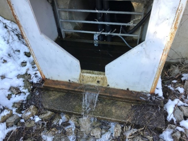
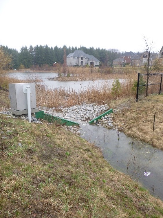
• Outlet measures water leaving Pond A through the outlet structure.
• Pond A Stage comprises measurements taken within Pond A near the outlet.
• Rain Gauge measures precipitation and air temperature.

Modelling

This model was set up using the EPA SWMM 5 software which is available free for use through the US EPA. The focus of this model was on Pond A and its surrounding catchment areas. The pond is mainly fed by the subdivision (Inlet 1) and the neighbouring Sheridan Nurseries property (Inlet 2), along with a much smaller area that drains directly into the pond. The model was developed and calibrated in three stages:

1. The model of Pond A and the small area that drains directly into the pond was set up using monitored inlet flow data and calibrated to monitored pond water levels and outlet flow.
2. Independent models of the subdivision and Sheridan Nurseries were set up and calibrated with Inlet 1 and 2 monitored flows respectively.
3. Once these elements were individually calibrated, they were combined into one model for the entire treatment train and its catchment areas.

Pond A Model Set-up and Calibration

Pond A is represented in the model using two storage nodes, one for the forebay, and one for the aftbay. For calibration of the pond, the majority of flow into the pond was incorporated using a time series for direct inflow into the forebay storage node. This time series includes combined inlet flow as well as direct precipitation. The direct precipitation volume was calculated using a surface area estimate based on the measured pond water level for that time step.

While the monitored inlet flow captures most runoff that would enter the pond, there is a small area that drains directly into the pond and would not have been measured at either inlet. Runoff from this area is modelled using a small subcatchment which receives precipitation measured from a nearby rain gauge. The precipitation from this rain gauge uses time series data for the same period as the monitoring data that was used to calculate inflow. Potential evaporation is modelled based on an air temperature time series from the MITG Rain Gauge using the Hargreaves method (Rossman L. and Simon M., 2022). Runoff from this subcatchment also enters the forebay to the pond. The pond water level was set to equal to the monitored water level at the start of the simulation.

To calibrate the model of the pond, the modelled water level within the aftbay storage node was compared to the monitored pond water level. Flow rates in the outlet pipe link were compared to flow that was monitored at a weir installed at the outfall of this pipe. For additional details on model set up, refer to Appendix B.

Treatment Train Model Set-up and Calibration

Pond A was set up as described above with the exception that direct precipitation was modelled using two impervious subcatchments, one with the surface area of the forebay and one with the surface area of the main pond. The two contributing catchments (Inlet 1 and Inlet 2) were calibrated individually based on monitored flow data for each station, then the design storm analysis was performed on the system as a whole.

The SWMM model for Inlet 1 (subdivision flow) used EPA SWMM’s built-in options to simulate LID controls such as a bioretention cell, permeable pavements, and soakaway pits. Parameters were based on information provided in the design or from literature (see Appendix B for the parameters that were used). The conveyance system was represented using a network of open channel conduits to represent the grass swales and circular conduits to represent the culverts. Junction nodes were located at the upstream and downstream of each driveway culvert and included a 15 centimetre offset above the swale invert of the upstream node to promote infiltration (Stantec, 2007a).

A survey with Differential Global Positioning System (DGPS) was conducted to provide accurate slopes for the swale network and elevations for relevant features within the treatment train. For elements that were not measured, information from the design drawings was used as necessary.

One limitation of EPA SWMM is that there is no option for representing rolled curb inlets, therefore smaller subcatchments were used (identified based on a drainage analysis conducted in PCSWMM; see https://www.pcswmm.com/Features for more information). Flow from these subcatchments was then directed to nodes along the conveyance network. One consequence of this was that the culverts needed to be modelled as larger than they are (1 metre diameter was used instead of 30 centimetres) to avoid being overwhelmed by flow being directed to the adjacent node, when in reality that flow would be distributed along the length of the swale.

Since pond design typically focuses on the extreme summer rainfall events, the model was run continuously using data for June through December from 2018 to 2020 (36 months). The calibration focused on peak flow and total volume for the biggest events with monitoring data. Total volumes for the entire modelled timeframe were also compared. Table 1 summarizes the calibration results for Inlet 1 (the subdivision) for selected events as well as the full dataset for summer and fall 2018 to 2020. The calibration for Inlet 1 results show that there is agreement between the observed and modelled total volume (within 10 per cent), but the model consistently overestimates peak flows for medium sized events. However, the modelled and observed peak flows are very similar for the two largest precipitation events in the dataset (July 17, 2019 and August 1, 2020) with only a 3 per cent and 6 per cent difference, respectively.

Table 1: Calibration summary for Inlet 1 catchment comparing observed and modelled peak flow and total volumes for select precipitation events. Infiltration estimated using Horton Method for modelled results.

Parameter	Flow for summer/ fall (2018 to 2020)	July 5 2018	July 16 2018	Aug 17 2018	July 17 2019	Aug 1 2020
Precipitation Depth (millimetres)	1229	20.2	29.6	16.8	42.0	75.2
Observed Peak Flow (litres per second)	613	112	138	96	613	515
Modelled Peak Flow (litres per second)	628	233	155	157	628	547
Observed Volume (litres)	11693924	194907	396948	206499	1086281	2773586
Modelled Volume (litres)	12328255	324397	478324	248579	1207254	2742403

Analysis

Once the EPA SWMM model had been set up and calibrated it was then used for three different analyses:

1. Design Storm Analysis was completed to inform on performance of treatment train during design storm events. It was done using the model of the entire treatment train and its catchment areas, and design storms generated using the same IDF parameters as the design model.
2. Seepage Analysis was completed to assess whether seepage from the pond was a driver of seasonally low pond water levels. It was done using the model of Pond A and the area that drains directly into it; Inlet 1 and 2 flows were represented using monitored data for the years 2017 to 2020.
3. Inlet Flow Analysis to better understand the influence of passing untreated flow from the Sheridan Nurseries property on the seasonal pattern of pond water levels. It was done using the model of Pond A and the area that drains directly into it; Inlet 1 and 2 flows were represented using monitored data for the years 2017 to 2020.

Design Storm Analysis

The goal of the design storm analysis was to compare peak flows for the calibrated EPA SWMM model of the treatment train with the 2007 design SWMHYMO model for 2 to 100 year events. This will help inform how the treatment train system as a whole performs relative to the design model, which was modelled without accounting for the LIDs (due to requirements at the time).

In addition to including the LIDs, the 2024 calibrated EPA SWMM model had other key differences from the 2007 design model including:

• Using the groundwater module to represent the observed inter-event flow.
• Using smaller subcatchments to direct water into the swale conveyance system, which was not explicitly modelled in the 2007 design model.
• The 2007 design model was developed using different software (SWMHYMO).

The design storms with 2 to 100 year return periods were generated using Dstorm, a free tool developed by a user on the OpenSWMM forums (Rossman L., 2022 accessed from https://sites.google.com/view/dstorm). The same IDF parameters were used as the original design model, along with the 6 hour Chicago rainfall distribution (same as for design model) (Stantec, 2007a). The water level in Pond A was set to 1.5 metre depth prior to the event, which corresponds to the elevation of the permanent pool.

Seepage Analysis

The seepage analysis was conducted to better understand the drivers behind the seasonal pattern in which the pond level stabilizes significantly lower than the permanent pool for much of the summer and fall. One possible reason why the pond level isn’t stabilizing at the permanent pool is because the pond liner may not be fully effective, causing seepage to the subsurface.

If seepage fully explains the seasonal pattern, then if the model is run with no seepage, we would expect the seasonal pattern to disappear and the pond to stabilize at or near the permanent pool throughout the year. If some seepage is occurring, but it doesn’t fully explain the seasonal pattern, it would likely be reflected in the shape of the recession curve when the water level in the pond is below the permanent pool elevation. If the pond level is below the permanent pool elevation, no water would leave the pond through the outlet structure. In this case, the recession curve would show the combined effect of evaporation and seepage.

To determine an estimate of seepage rate, the model was originally set up assuming no seepage was occurring. Then the seepage rate in the storage nodes was adjusted until the shape of the recession curves below the permanent pool level matched the monitored pond water level as closely as possible.

Inlet Flow Analysis

It is also possible that the runoff from the neighbouring Sheridan Nursery property which enters the pond through Inlet 2 is a driver behind the seasonal pattern observed in the pond. Specifically, the low water levels in Pond A in the summer and fall and near constant flow in the winter and spring. Inlet 2 flow data shows a similar pattern to the pond, with flow that is nearly continuous during the winter and spring, and very limited during the summer and fall.

According to the design report, Pond A was not designed to provide treatment for the Sheridan Nurseries runoff as this was not required. The pond had been designed to allow this water to pass through it (Stantec, 2007a). Therefore, to explore the influence of the Sheridan Nurseries runoff on the seasonal variability observed in the pond, an analysis was done to isolate the flow entering from the subdivision only. This analysis involved comparing three different modelled scenarios to the monitoring data. The modelled Pond A water levels and outflow for each scenario were then graphed to see if the same seasonal pattern is observed:

• Scenario a: Monitored flow data from both inlets, and a seepage rate as determined by the seepage analysis. This represents conditions that are closest to what is observed in the field.
• Scenario b: Only monitored flow data from Inlet 1, direct precipitation and modelled runoff from the surrounding subcatchment were used. This scenario was run with both the seepage rate determined by the seepage analysis as well as with seepage set to 0. This scenario where the pond is only receiving runoff from the subdivision represents the flow volumes that Pond A was actually designed to treat.
• Scenario c: The Inlet 1 flow time series was multiplied by a factor of 1.7. This factor was chosen because it results in the same total volume as the monitored total volume for both inlets combined. This scenario was run with both the seepage rate determined by the seepage analysis as well as with seepage set to 0. The model was run with this inflow (along with direct precipitation and runoff from the surrounding area) to determine whether the timing of flow entering the pond from the rural area has an impact independent of increasing the total volume.

Findings

Question 1: What insights can we gain from the EPA SWMM modelling exercise regarding the original design and its modelling process?

A design storm analysis was conducted to compare the results from a calibrated EPA SWMM model (which included the upstream LIDs) with the 2007 SWMHYMO design model (which did not include the upstream LIDs) (see Table 2). The analysis used the 6 hour duration Chicago rainfall distribution and the IDF parameters provided in the stormwater management report (Stantec, 2007a) to be consistent with the 2007 SWMHYMO design model.

Table 2: Design storm analysis peak flow results for 6 hour duration Chicago design storm.

Return Period (years)	Design Model			Calibrated Model
	Existing (Pre-development) (litres per second)	Pond A Outflow (litres per second)	Inlet 1 (litres per second)	Inlet 2 (litres per second)	Combined Inlet Flows (litres per second)	Pond A Outflow (litres per second)
2	550	40	483	23	506	33
5	1020	120	990	40	1030	81
10	1380	270	1339	57	1396	216
25	1860	500	1803	98	1900	435
50	2260	760	2113	142	2254	631
100	2650	1060	2439	196	2635	854

As shown in Table 2, the peak flows at the outlet of pond A are consistently less for the calibrated model than the design model predicted for the 2 to 100 year storms. For the 100 year storm the calibrated model’s peak flow is approximately 81 per cent of what the design model estimated. This suggests that it would have made a difference to include the LIDs in the design model, and that the pond is oversized.

Volume reductions provided by the up-gradient LIDs likely contribute to the pond’s low water levels observed in the summer and fall. Therefore, the design storm analysis might be a conservative estimate of the influence of the LIDs on peak flow performance for extreme events that occur during the summer and fall. This is because the design storm analysis assumed that the pond was at the permanent pool level at the start of the event, whereas monitoring suggests this would rarely be the case during the summer and fall. However, in order to be comparable to the design model, this analysis was strictly event-based and calibrated to summer data, it therefore does not represent the winter and spring conditions that monitored data shows result in the highest flows at the pond outlet, specifically snowmelt followed by rain on snow (Credit Valley Conservation, 2021).

Table 2 also shows the individual and combined inlet flows entering the pond for each of the return periods. This includes flow from Inlet 1, comprising the flow leaving the subdivision and all upstream LIDs, along with the flows contributed by the neighbouring Sheridan Nurseries property (Inlet 2). For all events, the combined inlet flows for the calibrated EPA SWMM model are within 10 per cent of the peak flows estimated for existing conditions by the design SWMHYMO model. Most of this flow is contributed from Inlet 1 despite it having a smaller catchment area. This makes sense since the catchment area for Inlet 2 did not undergo development and remains agricultural land with limited impervious cover. 

Although the design storm analysis suggests that the pond (as part of a treatment train) is exceeding design expectations with respect to peak flow control, the seasonal pattern observed in the monitoring data may exacerbate maintenance issues. For example, the stagnant water during the summer and fall may promote algae growth and encourage mosquitoes.

Summary: What insights can we gain from the EPA SWMM modelling exercise regarding the original design and its modelling process?

• The treatment train (including LIDs and Pond A) is exceeding performance expectations for control of design storms up to the 100 year event under summer conditions. Specifically, the calibrated model’s peak flow for the 100 year event is only 81 per cent of the flow that the design model predicted. This suggests that this pond might be oversized, and that the entire treatment train should be included in the water balance calculation for future design models in order to represent the conditions within the catchment more accurately.
• It is recommended to explore modelling approaches that better account for winter conditions in future design models. In the context of climate change, and intensified freeze-thaw cycles, rain on snow events may become more common. Even if flood control targets (100 year event) are still being met, changing winter conditions could result in water quality or erosion targets not being met more often.
• It is also recommended to consider the influence of season on flow and volume to properly understand annual water balances and reproduce the natural hydrologic cycle.

Question 2: What are the drivers of the seasonal pattern observed in the stormwater management pond?

Monitoring data revealed that water levels in Pond A follow a seasonal pattern where water levels are well below permanent pool level for much of the summer and fall, and outflow from the pond only occurs following extreme rainfall events. By contrast, flow is nearly constant during the winter and spring months (Credit Valley Conservation, 2021). 

This question focuses on understanding the relative impact of 2 possible drivers of this seasonal pattern: seepage rates and runoff from the neighbouring Sheridan Nurseries property.

If the above two drivers do not fully explain the seasonal pattern observed, this suggests that the seasonal pattern also reflects inaccuracies in the design water balance due to not factoring in the LIDs.

By running a continuous model of the pond using 36 months of monitored inlet data, it was possible to replicate the seasonal pattern described above. This pattern includes prolonged periods where precipitation generated no outflow and the pond water level stabilized below the permanent pool elevation, demonstrating the importance of seasonal and antecedent conditions in understanding the behaviour of the pond.

To better understand the drivers of this seasonal performance, different scenarios were modelled in terms of seepage rates and inlet flows (refer to the methods section on Inlet Flow Analysis for a description of these scenarios). These modelled scenarios also provided further insights into how seasons are reflected in overall flow volumes:

• Although only approximately 50 per cent of the total precipitation for the monitoring period occurred between January and June, for all model scenarios, 80 per cent or more of the total discharge from the pond was recorded during these months.
• Ninety per cent or more of the January to June discharge occurred from January to end of April across all model scenarios. This is not just the effect of the pond but reflects the upstream treatment train as well, since 84 per cent of total combined inlet discharge entered the pond between January to June.
• It was the winter months in particular that contributed the greatest proportion of total flow. For the combined inlets, and for all model scenarios, 58 per cent or more of the total discharge occurred from the start of January to the end of March. At both inlets, inter-event flow was observed during the winter and early spring (Credit Valley Conservation, 2021), which likely contributed to the importance of this time period for overall flow volumes and may be related to perched water table conditions.

Seepage Analysis Findings

The goal of this analysis was to determine if seepage is occurring in the pond, and if so, whether that seepage can fully explain the seasonal pattern that was observed.

The first step of the analysis was to test the assumption that there is no seepage in the pond, by setting the pond’s seepage rate to zero in the SWMM model and comparing the modelled results to the monitored data. When the seepage rate in the pond is set to zero:

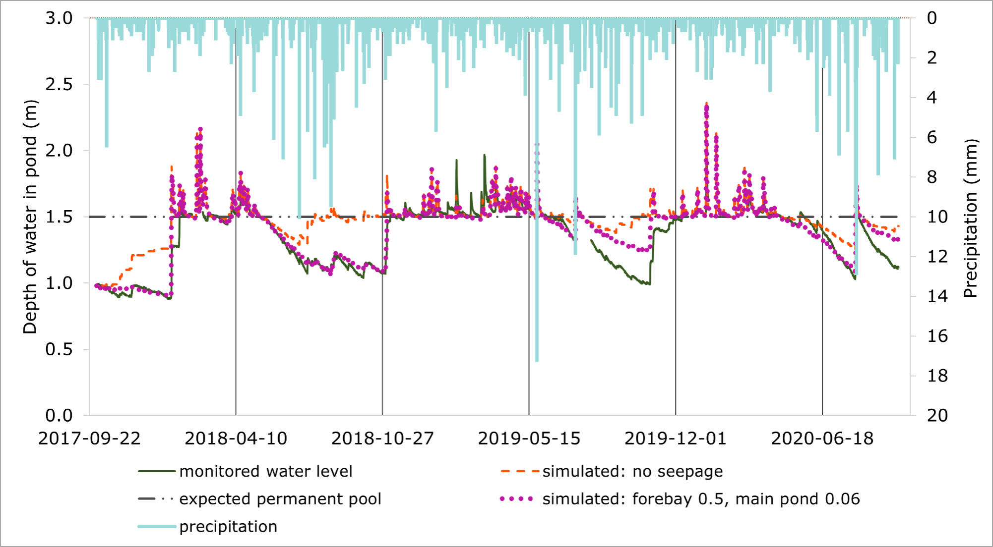
• The slope of the modelled recession curve is not as steep as what is observed in the monitored data (see Figure 3).
• Modelled flow occurs at the outlet to the pond more frequently compared to the monitored data: when the pond is modelled with no seepage there is some outflow for 27 of 36 total months whereas the monitoring data only recorded outflow for 18 of 36 total months.

These results suggest that some seepage is likely occurring in the pond, which helps explain the low water levels that were observed. However, seepage does not fully explain the seasonal pattern since there were still 9 months with no modelled outflow even when the seepage rate was set to zero.

The next step was to estimate the rate of seepage in the pond. To achieve this, the modelled rates of seepage were adjusted in both the main pond and the forebay, and the model results were compared to the monitored data for both the pond level and outflow. The CVC SWMM model results fit the monitored pond level best when the seepage rate in the forebay is set at a higher rate than in the main pond. It is not clear why the seepage rate might be greater in the forebay, though it might be due to differences in the underlying soil types or varying permeability of the clay liner. 

A hydraulic conductivity of 0.5 millimetres per hour in the forebay and 0.06 millimetres per hour in the main pond appeared to fit the slope of the recession curves the best:

• This resulted in the closest match in terms of the per cent of the time that water levels were at or above the permanent pool, with 45 per cent of the time for monitored data and 48 per cent of the time for the modelled data with this seepage rate.
• There were 22 months with some measured outflow for the modelled data, compared to 18 months for the monitored data.
• Although the pond water level modelled with this seepage rate matched the recession curves well for some years, the modelled recession curve is not steep enough to match the monitored data for others (Figure 3). It’s possible the seepage rate might change over time, potentially impacted by shifting patterns of sediment deposition and erosion.

This may also explain why flow still occurred more frequently in the model compared to the monitored data. For example, in the summer and fall of 2019 the modelled water level recedes less rapidly and as a result, a large precipitation event in late November results in flow for the model but not in the monitored data. 

Sheridan Nurseries Runoff (Inlet Flow Analysis) Findings

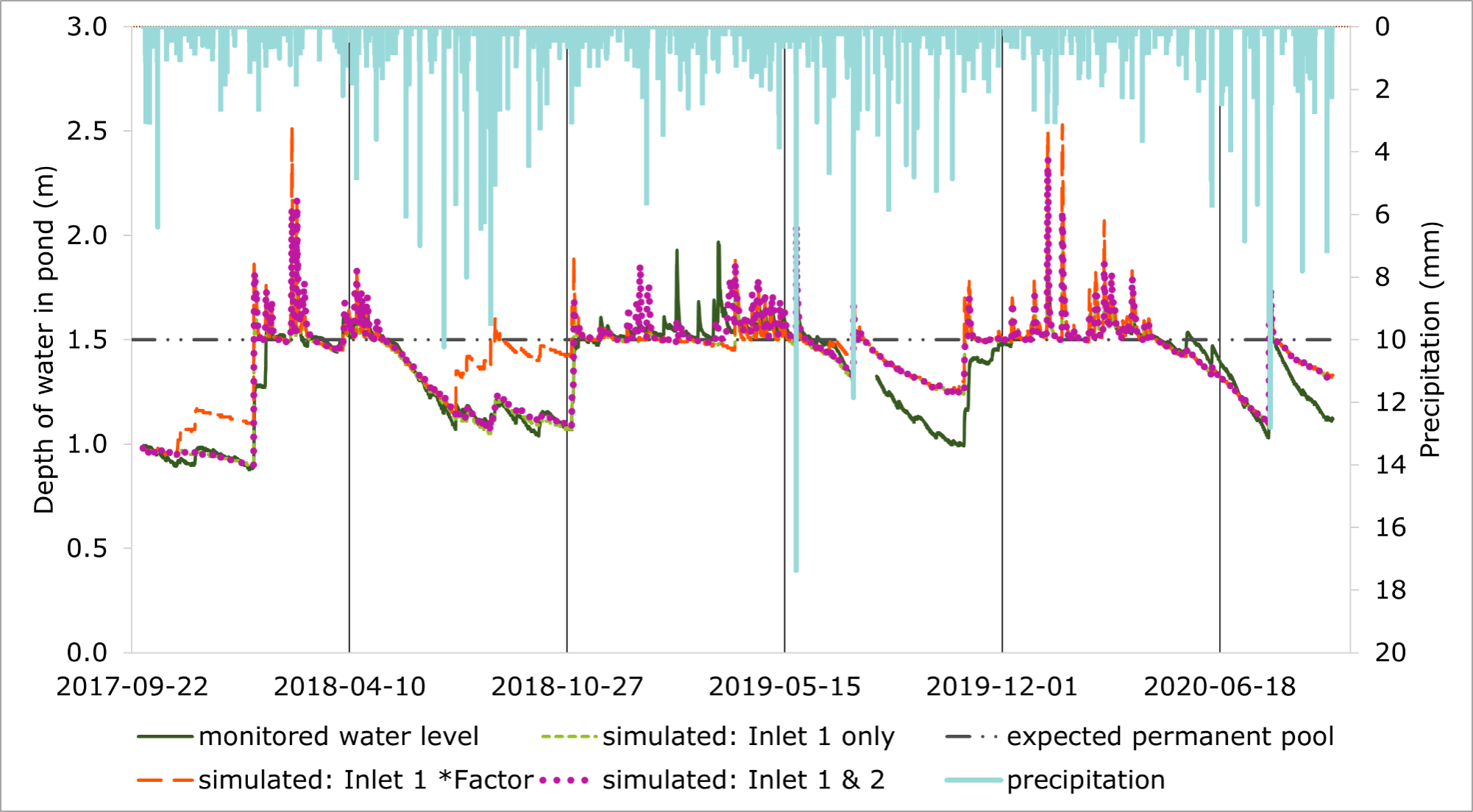
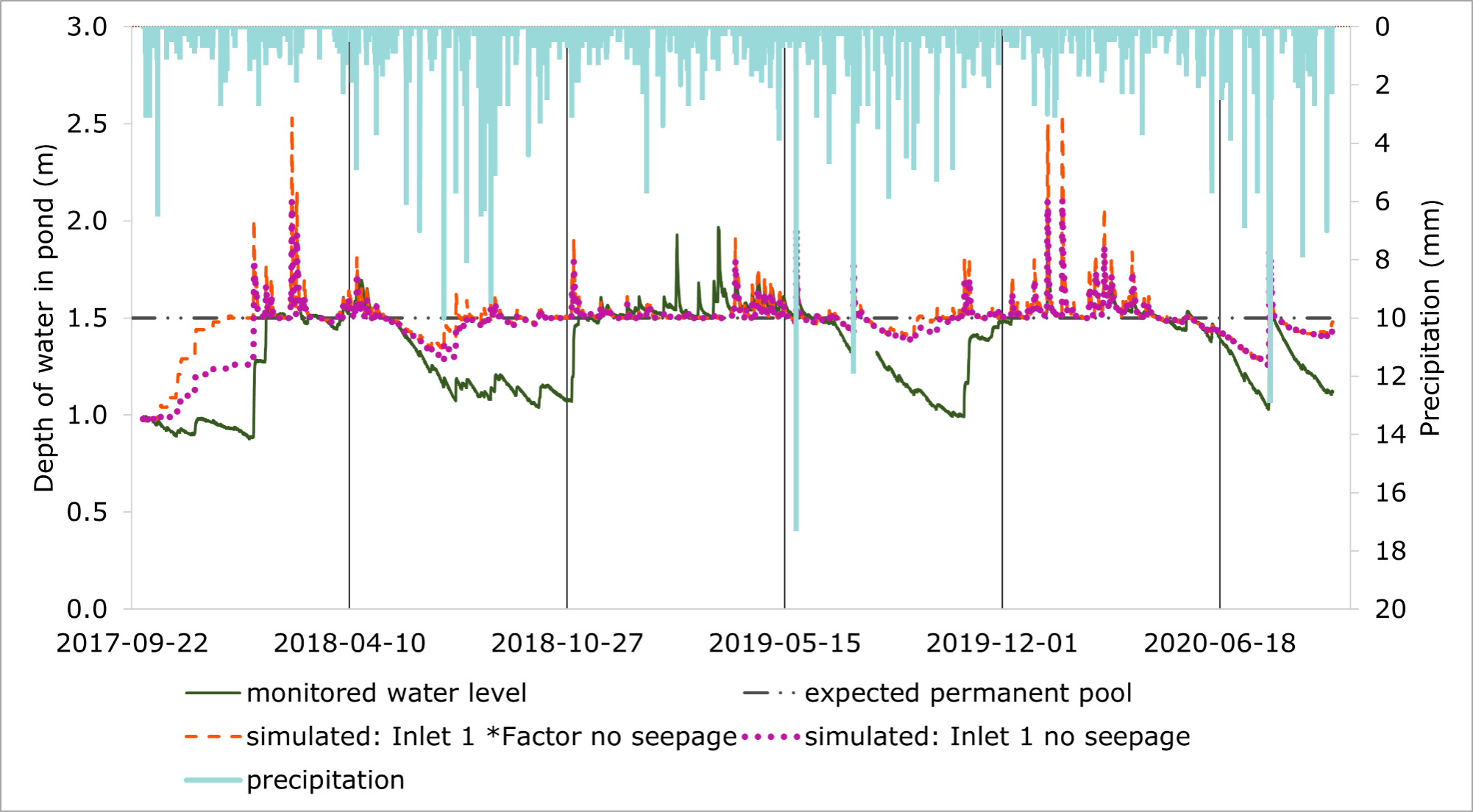
The design report indicates that 15.3 hectares of the neighbouring Sheridan Nurseries property are within the catchment area of the pond. This runoff from the Sheridan Nurseries property will influence the water level, outflow and seasonal pattern of the pond. However, runoff from this property does not require water quality treatment and therefore the pond is not designed to treat it but to “pass it” (Stantec, 2007a). To better understand the influence of passing runoff from the adjacent Sheridan Nurseries property, an inlet flow analysis was performed. This analysis consisted of running the calibrated EPA SWMM model of the pond with three different scenarios: (a) inflow from both inlets, (b) with inflow from the subdivision only (Inlet 1), and with (c) Inlet 1 multiplied by a factor of 1.7 (see Figure 4).

Multiplying Inlet 1 flow by 1.7 results in a total volume equivalent to Inlet 1 and 2 combined (the total volume entering the pond is the same as measured in the monitoring data only the timing changes). This was done to better understand the relevance of the timing of inflow as opposed to just the overall volume. It should be noted that the pond was not designed to treat the volume coming from the neighbouring Sheridan Nurseries property, so although it better reflects the volumes actually entering the pond, it is not what the pond was designed to treat.

The modelled pond water levels from all three scenarios were then compared to the monitored water level in the pond to understand the difference if there was no runoff contributed by the Sheridan Nurseries property:

• Scenario a: When the model is run with both inlets and a seepage rate of 0.5 millimetres per hour in forebay and 0.06 millimetres per hour in the main pond, the pond water level is at or above the permanent pool 48 per cent of the time.
• Scenario b: If the model is run with Inlet 1 inflow only and no seepage (the scenario that the pond was designed for) the pond water level is at or above the permanent pool level 63 per cent of the time, and 9 of the 36 months modelled had zero flow, all of which occurred between May and December.   
• Scenario c: If the model is run with Inlet 1 flow multiplied by a factor of 1.7 and no seepage the pond level is at or above pond permanent pool 70 per cent of the time and there is no flow for 7 of the 36 months modelled (Figure 5).

Comparing the results of these three scenarios suggests that “passing” runoff from the Sheridan Nurseries property is a contributing factor to the seasonal pattern of the pond because it impacts both the volume and timing of runoff. The neighbouring Sheridan Nurseries property has tile drainage which outlets to the Inlet 2 swale. Monitoring data recorded continuous flow entering the pond from Inlet 2 during the winter and spring (Credit Valley Conservation, 2021), which likely exacerbated the seasonal pattern observed in the pond. However, even without the contribution from the Sheridan Nurseries property the pond would not stabilize at the permanent pool level for parts of the year.

Summary: What are the drivers of the seasonal pattern observed in the stormwater management pond?

• Both seepage and flow from the Sheridan Nurseries property appear to contribute to the seasonal pattern observed at Pond A.
• The seasonal pattern is not exclusively driven by these site specific factors. Even if these factors are removed from the model there are still 7 months with no flow and the pond did not stabilize at or above the permanent pool 30 per cent of the time.
• This suggests that some of the monitoring results summarized in the main report, Stormwater Management Performance Summary: Meadows in the Glen Residential Subdivision, can be generalized to other treatment train and wet pond scenarios, however the effect may be less extreme.

Question 3: What challenges and lessons can be learned from modelling a site with a treatment train stormwater management approach?

Challenges encountered during the calibration process

There were two main challenges with calibrating the EPA-SWMM Model of the subdivision (Inlet 1):

1. The modelled results were flashier, but exhibited lower overall volumes compared to the observed data.
   • Solution: To increase the volumes for the modelled events, the groundwater module in EPA SWMM was used to simulate interflow. This helped improve the volume estimate for the modelled results. The following observations support the interpretation that interflow contributes to the overall flow volumes:
     • Field observations and monitoring data showed prolonged flow between events at certain times of year.
     • Monitored groundwater levels in the subdivision were typically more than nine meters below ground surface, so baseflow contributions from the regional groundwater system are unlikely.
     • Soil data shows variable permeability in the shallow subsurface; in some locations lower permeability layers were found at approximately 0.8 to 1.5 metres depth (Terraprobe, 2007).
2. The model overestimated peak flows for small and medium events while underestimated peak flows for larger events (those with greater than 2-year return period) when compared to monitored data. It was determined that the model was overestimating infiltration during large high intensity events, however adjustments to impervious cover and soil infiltration parameters did not sufficiently increase the peak flows during these events.
   • Solution: A better fit for precipitation events with greater than 2 year return period was found by comparing different approaches (Green and Ampt, Curve Number, and Horton Method) for estimating infiltration. The best fit for small to medium events was achieved when using the Green and Ampt method for estimating infiltration, however the best results for the largest precipitation events were achieved with the Horton Method. For the purpose of a design storm analysis, the results from the Horton Method were considered the most suitable because of the improved accuracy during large events. The results of the comparison of the Green and Ampt and Horton Method are summarized in Table 3.

Table 3: Comparison of Inlet 1 (subdivision) observed peak flows with modelled results using different approaches to estimate infiltration.

Precipitation Event Date	Precipitation Depth (millimetres)	Duration (hours)	Observed Peak Flow (Litres per second)	Modelled Peak Flow Green and Ampt Method (Litres per second)	Modelled Peak Flow Horton Method (Litres per second)
July 17, 2019	42	2.8	613	230	627
August 1, 2020	72.6	13.2	515	163	548

Lesson Learned: It’s important to use longer term monitoring datasets for calibration purposes wherever feasible, and ensure that a variety of event sizes are captured:

• If only one year of monitoring data (2017 to 2018) were used for calibration of the MITG subdivision model it would have appeared that the model was consistently overestimating peak flows. 
• It was only when the model was compared to an additional two years of monitoring data (2018 to 2020) that it was observed that the model of the subdivision dramatically underestimated the peak flows for some larger precipitation events (those with greater than 2 year return period).
• Without having a longer dataset to use for calibration the overestimation of infiltration during larger events would not have been recognized.

Challenges related to missing design details

There were also difficulties with developing the model of the subdivision that related to the design and the information that was provided in the drawings and design brief. Two main challenges that related to the level of detail provided in the design documents were:

1. Details relating to subsurface layers for LID practices were missing from design drawings meaning that assumptions had to be made in the model development. For example, the thickness of subsurface layers and the specific materials used were missing or difficult to interpret for some features such as the permeable pavement.
   • Recommendation: When reviewing and approving LID designs, consider whether adequate details are included clearly to facilitate accurate modelling if needed in the future. These details could also be important for monitoring and/or operations and maintenance activities required to ensure ongoing performance as designed. 
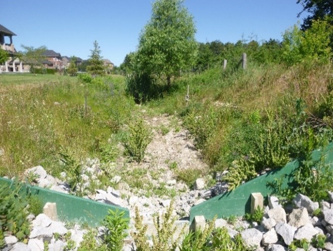
2. Some elements of the design lacked information on how they were expected to function and were therefore difficult to model. For example, flow in the upstream swale network is supposed to be diverted into the bioretention cell using a small grass berm. Without this berm, flow would just continue straight and follow the swale network to the pond. The design dimensions and expected proportion of the flow to be diverted by this berm were not clearly documented and field tests would have been challenging to implement. Field observations showed that the bioretention cell was receiving little if any flow diverted from the swale network.
   • Model Limitations: For this model, a conservative approach was taken by routing only the road runoff that would enter the facility directly via the rolled curb inlet to enter the bioretention facility, so as not to over-estimate the impact the bioretention cell would have on overall performance.
   • Recommendation: Future designs should better document how vaguely defined design elements such as this berm are expected to function, especially when they provide a key function such as diverting flow into a stormwater management practice.

Specific limitations of EPA SWMM

Some of the challenges encountered during development of the model relate to the specific limitations of EPA SWMM:

1. There is no option in EPA SWMM to represent conveyance features that receive flow throughout their entire length, such as via a rolled curb inlet. Instead, flow must enter conveyance systems at specific nodes. This made it difficult to represent the swale network, which received flow from the shoulder and sidewalk of the road via a rolled curb along its entire length.
   • Model Limitations: Assumptions had to be made when deciding which nodes to direct the flow from contributing subcatchments into. The length of swale where water has an opportunity to infiltrate is therefore not accurate. To reduce the impact of this limitation, smaller subcatchments were used. However, the smaller subcatchments and the requirement for multiple nodes increased the complexity of the model. Concentrating the inflow at individual nodes also resulted in overloading of culverts in some cases. To address this, the culverts had to be made larger in the model than they were in reality.
2. EPA SWMM has a groundwater module, however it doesn’t allow groundwater flow between separate subcatchments. This makes it challenging to represent return flow and interflow where water might infiltrate in one subcatchment and return to surface flow in another subcatchment.
   • Model Limitations: Inter-event flow was observed to make up a significant portion of the water balance at Meadows in the Glen, especially in the winter and spring. Although interactions with the regional groundwater system are not believed to occur at Meadows in the Glen due to the depth of the water table (9 metres or more), perched water table conditions in the winter and spring likely contribute to inter-event flow. Modelling this was challenging because smaller subcatchments had to be used as discussed above.
     • For the purposes of the design storm analysis, the model was calibrated to summer and fall events where the influence of interflow was observed to be less significant.
   • Recommendation: Where extensive interaction between LIDs and groundwater are expected it may be preferable to use a different modelling software. In particular, an integrated surface-groundwater model such as Mike-SHE or Hydrogeosphere might be preferable when complex groundwater interactions are expected (Matrix Solutions Inc., 2022).

Summary: What challenges and lessons can be learned from modelling a site with a treatment train stormwater management approach?

• The modelling process encountered a variety of challenges related both to specific site conditions, design details that were missing or unclear and the specific limitations of the modelling software. These limitations to the model should be kept in mind when interpreting the results.
• In this study, the Green and Ampt method for estimating infiltration was found to overestimate infiltration during large events (those with greater than a two-year return period). It is recommended that further comparisons and exploration of the suitability of different approaches for estimating infiltration depending on the purpose of the model.
• Another lesson learned is that it is important to ensure that an appropriate level of clarity and detail is included in future design drawings and documentation to support potential modelling, monitoring, operations and maintenance activities.

Conclusions and Recommendations

Site Characterization and Design

The modelling study revealed the importance of detailed site characterization, and that it is important to consider how site specific factors might influence the performance of the stormwater management treatment train during the design stage. It is also important that the design model includes all stormwater management practices (such as LIDs) to get an accurate idea of how the system as a whole will perform.

Conclusions:

1. The treatment train (including LIDs and Pond A) is exceeding performance expectations for peak flow control of design storms up to the 100 year (summer) event.
2. Due to the omission of the contributions of LIDs in the water balance calculations, the design may have overestimated the amount of water entering the pond, especially in the summer and fall seasons when pond water levels are very low. This suggests that the pond might be oversized.
   • Although both seepage and passing of flow from the Sheridan Nurseries property contributed to the observed seasonal pattern, they do not appear to fully explain the low water levels that were often observed in the pond (see discussion of Question 2: Drivers of seasonal performance of Pond).
   • While excluding LIDs from the water balance is a conservative approach, it may lead to a design model that does not accurately reflect site conditions, potentially causing unexpected asset management issues related to stagnant pond water.
3. Site specific factors can affect the performance of stormwater management practices and may be exacerbated by seasonal influences. These factors may include, but are not limited to, perched water table conditions, permeable and erodible soils, passing water from nearby areas with different flow regimes and interactions with groundwater.

Recommendations:

1. Including the entire treatment train in the design model is recommended for future stormwater pond designs to better reflect catchment conditions. Caution is advised when modelling stormwater management practices on private property, as uncertainty surrounding their long term maintenance can have consequences on the water balance.
2. In light of climate change, intensified freeze-thaw conditions and possibility of more frequent rain on snow events, it is also suggested that future design models explore approaches to better account for differences in performance under winter versus summer conditions to ensure water quality and erosion control targets are met.
3. More detailed site characterization could help identify site specific factors such as soil conditions and perched water table conditions so they can be better represented in design models. 

Modelling Recommendations

Developing a calibrated EPA-SWMM model for Meadows in the Glen involved a variety of challenges, limitations and lessons learned. These challenges lead to the following key recommendations: 

1. Recommend additional comparisons of infiltration estimation methods (such as Green and Ampt, Curve Number and Horton Method) for subdivision scale projects with long term monitoring datasets to help determine the most suitable method for use in future treatment train design models. 
2. Recommend using longer term monitoring datasets for calibration purposes wherever feasible and ensuring that a variety of event sizes are captured.

References

Credit Valley Conservation. 2021. Stormwater Management Performance Summary: Meadows in the Glen Residential Subdivision. Sustainable Technologies Evaluation Program. Ontario. https://sustainabletechnologies.ca/app/uploads/2021/12/rpt_mitgreport_FINAL_20211125.pdf

Matrix Solutions Inc. 2002. Advantages of Integrated Groundwater-Surface water Modelling Webinar.

Rossman L. and Simon M. 2022. Storm Water Management Model User’s Manual Version 5.2 USEPA.

Stantec (Kitchener). 2007a. The Meadows in the Glen Subdivision, Final Stormwater management and Low Impact Development Strategy Report, Glen Williams, for Intracorp Project (The Meadows in the Glen) Ltd.

Stantec (Kitchener). 2007b. The Meadows in the Glen, Environmental Implementation Report, Glen Williams, for Intracorp Project (The Meadows in the Glen) Ltd.

Terraprobe. 2007. Geotechnical Investigation Proposed Residential Subdivision “The Meadows in the Glen” Part of lots 20 &21, Concession 10 Town of Halton Hills Regional Municipality of Halton.

Appendix A: Monitoring Approach

Monitoring was conducted at 4 stations located around Pond A: Inlet 1, Inlet 2, Outlet and Pond A Stage from 2017 to 2020.  Inlet 1 and Pond A Outlet have been monitored starting in 2015, Inlet 2 starting in 2016 and Pond A Stage starting 2017.  Monitoring was also conducted at Tributary F, in groundwater wells around the subdivision, and at the outlet of Pond B. However, this data will not be presented in the report. The monitoring stations that will be focused on in this report are:

• Inlet 1 measures runoff from the MITG subdivision and the up-gradient LID treatment train.
• Inlet 2 measures runoff from the adjacent rural property and a small portion of the subdivision.
• Outletmeasures water leaving Pond A through the outlet structure.
• Pond A Stagecomprisesmeasurements taken within Pond A near the outlet.
• Rain Gaugemeasures precipitation and air temperature.

The monitoring infrastructure for these stations (with the exception of the rain gauge) is shown in Figures A1-A4.

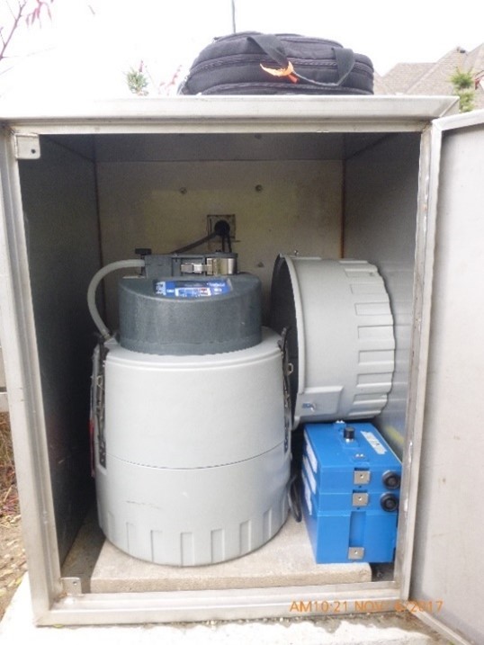
The details of the monitoring and inspections conducted at each station are summarized below in Table A1. The monitoring approach has been adapted over time in response to observations made with respect to the performance of Pond A; this has resulted in introducing new initiatives such as winter monitoring and pond stage monitoring. The standard equipment configuration is shown in Figures A5 and A6 including an automatic sampler, level logger, and calibrated weir to convert level measurements to flow.

Table A1: Summary of monitoring type, purpose and details for monitoring stations located at Pond A.

Monitoring Type	Monitoring Purpose	Stations Monitored	Equipment Used	Details
Precipitation and Air Temperature	Determine precipitation amounts.	Rain Gauge	Hydrological Services TB3 rain gauge and Sutron data logger	Remotely monitored weekly and calibrated in the spring/fall.
Continuous Flow	Determine peak flow and runoff volumes entering and leaving the pond.	Inlet 1, Inlet 2, Outlet	ISCO 2150 area-velocity loggers and compound weirs	Downloaded and calibrated with manual measurement on approximately monthly basis.
Continuous Pond A Water Level	Characterize seasonal pond level fluctuations and drawdown times with respect to permanent pool.	Pond A Stage	ISCO 2150 area-velocity loggers and fixed stage	Downloaded and calibrated with stage reading on approximately monthly basis, initiated 2017. Level sensor and stage installed in aftbay of pond near the outlet.
Winter Flow	Obtain flow data when there is risk of freezing damage to ISCO 2150 loggers.	Inlet 1, Inlet 2, Outlet	HOBO water level loggers and compound weirs	Monitoring plan did not initially include winter monitoring, initiated winter of 2016-2017.
Maintenance Inspections	Track condition of LID features and identify maintenance issues.	Throughout subdivision	Camera and checklist	Completed every few months for bioretention cell, permeable pavers and grass swales. Only completed once at Pond A.
Bathymetric Survey	Determine baseline sediment build up in Pond A.	Pond A	Performed by consultant	Completed September 2017.

Appendix B: Model Set-up Details and Parameters

The overall Model Setup is shown in Figure B1, and details for how the model was developed are provided below.

SWM Pond A

• Pond A is represented in the model using two storage nodes, one for the forebay, and one for the aftbay.
  • Both storage nodes use tabular storage curves that were developed based on storage area and depth-discharge information provided in the design report (Stantec, 2007a)
  • The two storage nodes are connected by a trapezoidal weir used to represent the berm that separates the forebay and aftbay.
• The Pond A outlet is represented with four separate links that connect to a single node which is then connected to the outfall by another link:
  • Two orifice links are used to represent the outlet structure, an upper and a lower one.There is also a ditch inlet catchbasin and a spillway that are both represented using outlet links.These are all directed to a node representing the ditch inlet catchbasin manhole.
  • This node connects to a conduit link that represents the outlet pipe which is in turn connected to the outfall.

Subdivision (Inlet 1)

Subcatchments:

• Slope was based on the design document (Stantec, 2007).
• Infiltration parameters informed using and grain size descriptors from the geotechnical study (Terraprobe, 2007) and the Soil Plant Air Water (SPAW) soil characteristics tool developed by the United States Department of Agriculture https://irrigationtoolbox.com/NEH/UserGuides/SPAW%20User%20Guide.pdf
• Subcatchment delineation was done initially using PCSWMM’s built in functionality and a Digital Elevation Model.
• The subcatchment delineation was refined based on interpretation of the design and informed by field observations and monitoring data.

LID Controls:

• Soakaway pits were located on most properties, they were assigned to the subcatchment that contained backyard of the property, if that was a different subcatchment than the roof, then the impervious area of that roof would be reassigned to the subcatchment of the backyard.
• Seperate subcatchments were used to represent the roads, with runoff directed to permeable pavers and then into the enhanced swale network via the nearest nodes.

Drainage Network:

• Enhanced Swales were modelled using open channel conduits (dimensions and slopes based on combination of design and DGPS survey).
• DGPS survey was used to measure elevations of inverts and tie these into key monitoring infrastructure used for calibration.
• Nodes upstream and downstream of each driveway with 15 centimetre offset at the upstream node
• Culverts represented by closed round conduits.
• Runoff from road is directed to upstream node of swale network (no option for rolled curb)
• Seepage loss parameters informed by geotechnical study (Terraprobe, 2007).

Sheridan Nurseries (Inlet 2)

• Simplified representation with single subcatchment
• Impervious area based on GIS analysis
• Soil parameters based on information from geotechnical study (Terraprobe, 2007)

LID Parameters

The LID Parameters were sourced from a combination of the design document (Stantec; 2007a), the geotechnical report (Terraprobe 2007), or sourced from reference values in the SWMM Help document or other literature sources.  The parameters that were used for the LID Controls are summarized for the different layers in Table B1 through Table B5.

Table B1: Surface Layer Parameters.

LID Control:	Soakaway Pit	Bioswale	Permeable Pavement
LID Type:	Infiltration Trench	Bio-Retention Cell	Permeable Pavement
Berm Height (mm):	0	0.3	0
Vegetation Volume Fraction:	0	0.0	0
Surface Roughness (Mannings n)	0.027	0.4	0.1
Surface Slope:	0	1	2

Table B2: Storage Layer Parameters.

LID Control:	Soakaway Pit	Bioswale	Permeable Pavement
LID Type:	Infiltration Trench	Bio-Retention Cell	Permeable Pavement
Thickness (mm)	1000	390	500
Void Ratio	0.625	0.78	0.75
Seepage Rate (mm/hr)	36.068	36.068	36.068
Clogging Rate	0	0	0

Table B3: Drain Parameters.

LID Control:	Soakaway Pit	Bioswale	Permeable Pavement
LID Type:	Infiltration Trench	Bio-Retention Cell	Permeable Pavement
Flow Coefficient:	0	1.25	0
Flow Exponent:	N/A	0.5	N/A
Offset (mm)	N/A	190	N/A

Table B4: Soil Layer Parameters.

LID Control:	Bioswale	Permeable Pavement
LID Type:	Bio-Retention Cell	Permeable Pavement
Thickness (mm):	210	0
Porosity:	0.437	N/A
Field Capacity:	0.105	N/A
Wilting Point:	0.047	N/A
Conductivity mm/hr:	29.5	N/A
Conductivity Slope	53.55	N/A
Suction Head (mm)	2.4	N/A

Table B5: Pavement Layer.

LID Control:	Permeable Pavement
LID Type:	Permeable Pavement
Thickness (mm):	80
Void Ratio:	0.15
Impervious Surface Fraction:	0
Permeability (mm/hr)	100
Clogging Factor	0
Regeneration Interval (days)	0
Regeneration Fraction	0