

London Residential Smart Hybrid Heating Pilot: System Performance Analysis
Prepared By: The Sustainable Technologies Evaluation Program (STEP) of the Toronto and Region Conservation Authority (TRCA)
December 2023
Contact Information: step@trca.ca
Executive Summary
This report provides performance analysis results from eight homes participating in the smart hybrid heating pilot conducted in London, ON, by Enbridge Gas Inc. and London Hydro. The full pilot consisted of 105 homes, with systems installed in late 2021. The systems included an air-source heat pump (ASHP), a back-up furnace, and a smart-switching thermostat.
In some cases, the existing furnace was used, and in others, a new furnace was installed. The ASHPs replaced the air-conditioning units used in the homes and provided all the homes’ cooling needs. The ASHPs also provided a portion of the homes’ heating needs.
The smart-switching thermostats were configured such that the ASHPs only operated when they were estimated to be the lowest cost heating option when compared to the furnace, based on the time-of-use (TOU) electricity bracket and the expected ASHP efficiency. This typically meant that the ASHPs had more frequent operation in off-peak or mid-peak TOU brackets, and/or in milder outdoor temperatures. The furnace and ASHP never ran at the same time.
Data collection systems were deployed in the eight study homes to determine the ASHP power consumption and furnace gas consumption post-retrofit. Regression analysis was used to determine savings. Post-retrofit data was analyzed from June 2022 to April 2023. Key metrics from the study homes are summarized in Table 1. Table 1 shows that the ASHPs:
- reduced the utility bills of the home,
- provided most of the home heating needs,
- reduced carbon emissions,
- operated with a high-efficiency, and
- did not significantly increase the aggregated peak electricity demand of the homes.
Table 1. Summary of key metrics for the 8 study homes
| Parameter | Unit | Minimum | Maximum | Average |
| Heating Mode Utility Savings | $ % | 37 7 | 143 27 | 71 15 |
| Cooling Season Utility Savings | $ | -16 | 245 | 94 |
| Heating Season Carbon Reductions (Based on Marginal Electricity Grid Emission Factor) | TCO2e % | 0.28 18 | 1.06 54 | 0.64 40 |
| Cooling Season Carbon Reductions | TCO2e | -0.03 | 0.33 | 0.15 |
| Fraction of Heating Provided by ASHP | % | 25* | 74 | 58* |
| Seasonal Coefficient of Performance | W/W | 2.1 | 3.3 | 2.8 |
| Annual Peak Demand Increase Post-retrofit | % | -15 | 25 | 2 |
*Only 25% of the heating was done by the ASHP in one home because of an issue that caused the ASHP to be off entirely for more than half the heating season. This home was an outlier. Not including this outlier, the minimum fraction of heating provided by the ASHP was 53%, and the average was 63%.
Three key areas of potential improvements for both operating cost and carbon emissions reductions were identified:
1. Avoiding unnecessary defaulting to the furnace
The monitoring data showed that the ASHPs generally only operated when the control algorithm predicted that they were the more economical option. However, the fact that the smart switching thermostats were web-connected devices that allowed a user to change configuration parameters, meant that the furnaces operated somewhat more frequently than expected in the homes (to varying degrees) and this reduced carbon and cost savings. Thermostat manufacturers should explore ways to avoid unnecessarily defaulting to the furnace, specifically when there is a web-connectivity issue.
2. Improving ASHP sizing and selection to achieve more optimal savings
Across all homes, the ASHP was predicted to remain the most economical option in an off-peak TOU bracket for outdoor temperatures down to below -16°C. Utility bill savings potential is therefore greatest in installations where the ASHP is sized to cover as much of the heating load as possible within the constraints of the home and budget.
However, on average, the ASHPs in this study did not have enough capacity to heat the homes below an outdoor temperature of -5°C (it varied between -0.8°C and -13.3°C in different homes) and the furnaces had to often be used in cold temperatures even though they were predicted to be less economical. This reduced savings. In half of the eight study homes, the ASHPs were effectively not able to do smart switching because they were not sized to have enough heating capacity in cold temperatures. They switched between furnace and ASHP at the same outdoor temperature across all TOUs.
There are different considerations for sizing including both upfront costs and the technical constraints of the home. Overall, contractor training is needed to help ensure optimal system sizing, and that the available sizing and selection tools are applied to right-size ASHPs to meet homeowner needs.
3. Considering carbon reductions in the thermostat control algorithm
The smart-switching thermostats sought to optimize operating cost reductions. It would be helpful for homeowners if smart-switching thermostats were equipped with a user-selectable mode of operation that considered both cost and carbon savings optimization. The thermostats in this study had this function but the pilot focused on cost benefits, and homeowners did not use the carbon optimization feature.
It may be the case that notable increases in carbon reductions are achievable for small increases in operating cost when compared to a “cost-only” optimization approach. It would be further beneficial if marginal emissions factor data were published in real-time from the IESO, such that this could be an input to future thermostat algorithms.
One home exemplified the potential benefits of smart-switching. In this home, electricity consumption in a peak TOU represented only 2% of the total ASHP electricity consumption such that the ASHP was driven mainly with lower cost electricity. This factor, combined with an efficient inverter-driven ASHP that had sufficient cold temperature heating capacity, allowed it to achieve the greatest heating season cost savings in the study ($143) while also reducing furnace gas consumption by 72%.
A recommendation for future work is that more research on the demand impacts of electrifying home heating loads with hybrid systems is needed. In this study, the home heating loads were 58% electrified on average and the aggregated annual peak electricity demand of the homes increased by only 2%.
It would be helpful for broadscale planning to better understand (based on real-world data) how peak demand is impacted by hybrid systems on a broadscale and how factors like the ASHP efficiency, ASHP sizing, and control algorithm influence peak demand.
From a demand perspective, it is also prudent that smart switching thermostats be equipped with the ability to participate in future utility demand side management programs that may seek to actively curtail ASHP electricity consumption during times of grid congestion. Active demand management may help to overall increase the total penetration of ASHPs on the grid while mitigating potential negative grid impacts.
Readers are encouraged to review the study limitation provided in Section 14.10 of this report. Overall, this study builds confidence in ASHP technology, and provides further data and analysis to show that they are indeed high-performance devices that can reduce carbon emissions and homeowner utility costs.
Table of Contents
- Introduction
- Systems Overview
- Data Overview
- Analysis Procedure
- Results: Baseline Furnace Consumption
- Results: Gas Energy Savings
- Results: ASHP Electricity Consumption in Heating Mode
- Results: Fraction of Heating from ASHP
- Results: Estimated As-installed SCOP
- Results: Net Cost Savings
- Results: Electricity Demand Changes
- Results: Net Carbon Reductions
- Results: Summary
- Discussion
- Conclusion
- References and Endnotes
- STEP
- Notice
- Acronyms
- Acknowledgements
1 Introduction
The residential smart hybrid heating pilot commenced in late 2021 in London Ontario, as a partnership between London Hydro and Enbridge Gas Inc. The program provided $3,200 to 105 homeowners to install a smart hybrid home heating system. These systems included an air-source heat pump (ASHP), a back-up furnace (new or already existing in the home), and a smart-switching thermostat.
ASHPs are an alternative home heating and cooling option. They can completely replace a traditional furnace in some homes when used with electric back-up, or they can utilize a furnace as back-up heating to create a hybrid heating system. In heating mode, ASHPs extract renewable heat energy from cold outdoor air which is then used to heat the home. Modern cold-climate versions can do this even in extremely cold conditions.
ASHPs use the same basic technology as an air-conditioner, only with upgraded components, and with the ability to operate “in reverse” to provide both heating and cooling. ASHPs are a key technology for reducing, and eventually eliminating carbon emissions, from home heating provided that they are powered with a clean electricity grid. Some models can achieve efficiencies on the scale of 3x that of conventional equipment and this may also drive lower utility costs for homeowners.
A smart-switching hybrid system is designed to optimize operating cost reductions for homeowners. The cost to operate an ASHP will vary with the outdoor temperature (since ASHP efficiency decreases as it gets colder outside) and the time-of-use (TOU) electricity bracket. The smart-switching thermostat is web-connected and evaluates the ASHP cost of operation in real-time to determine whether it is expected to be lower cost compared to the furnace. It then selects the ASHP to provide heating whenever it is expected to be the lowest cost.
The smart-switching thermostat effectively sets an outdoor temperature threshold for each TOU bracket. Above the threshold, the ASHP is more economical to operate. Below the threshold, the furnace is more economical to operate. These thresholds are termed the economic balance point temperatures (EBPTs) and, again, there is one for each TOU bracket.
ASHPs may be further constrained by the thermal balance point temperature (TBPT). Below the TBPT, the ASHP does not have enough capacity to meet the home heating load and the furnace is used even if the ASHP is expected to be more economical. The TBPT will vary with the home heating load, the nominal capacity of the installed ASHP, and the capacity maintenance of the ASHP into cold-temperatures. Put simply, the smart switching thermostat selects the ASHP to provide heating whenever it is expected to be the lowest cost and it has enough capacity. Otherwise, the furnace is selected.
This report provides performance analysis from eight homes participating in the pilot. The data monitoring systems in the study homes were installed in 2022. They measured the heat pump power consumption and furnace gas consumption. Weather data was collected from a local weather station. Regression analysis was used to create baseline furnace energy consumption models from which the gas savings could be calculated. Cooling mode savings and demand savings were also evaluated using hourly whole-home electricity data from London Hydro.
The process of determining savings from an energy efficiency measure (EEM) is termed measurement and verification (M&V). Energy savings associated with an EEM are not directly measurable. Energy savings are the difference between the energy consumption that would have occurred had the EEM not been implemented, and the energy consumption that did occur. This necessarily means that savings is an estimate because the calculation procedure needs to make assumptions about something that did not actually happen.
The furnace gas energy consumption that would have occurred without the ASHP was estimated using regression analysis of the furnace submeter data, and considering only those days when the ASHP electricity consumption was negligible. The use of regression analysis to define baseline energy consumption is a common methodology deployed in the M&V of EEMs in large buildings, based on the International Performance Measurement and Verification Protocol (IPMVP), and is equally as valid in homes.[1] The modelled baseline gas consumption was compared against the actual gas consumption of the homes to determine heating mode savings.
Key performance metrics were calculated for each home, among them were:
- the as-installed seasonal coefficient of performance (SCOP),
- the fraction of heating provided by the ASHP,
- the net economic savings in heating and cooling mode,
- the net carbon reductions, and
- the change in the peak whole-home electricity demand.
2 Systems Overview
The systems participating in the monitoring are shown in Table 2. Two systems that had been monitored were omitted from the analysis and are not listed here. In one case, the homeowner moved, and in the other, data losses were substantial, and this resulted in the home not being sufficient for analysis.
Brand or model numbers are omitted from the table because the study was not designed (nor was it intended) to be a comparison across different ASHP brands. While the models/brand of the former A/C units were collected, the units were very old in most cases and data on the SEER was not available to the research team.
Table 2. Overview of HVAC systems included in the monitoring study
| Identifier | Furnace Capacity [kBTU/hr] | Furnace AFUE [%] | Nominal Capacity of Former A/C Unit [RT] | Nominal Capacity of New ASHP [RT] | ASHP HSPF (Region IV) | ASHP Capacity at -8.3 oC. [kBTU/hr] | ASHP SEER | ASHP Compressor Type |
| H1 | 45 (New) | 96% | 2 | 2.5 | 9.5 | 17,900 | 17 | Two-stage |
| H2 | 60 (Existing) | 95% | 1.5 | 3 | 10.0 | 24,000 | 18 | Inverter |
| H3 | 60 (Existing) | 95% | 2 | 2 | 9 | 14,000 | 17 | Two-stage |
| H4 | 88 (New) | 96% | 3 | 3 | 9.5 | 23,400 | 17 | Two-stage |
| H5 | 60 (New) | 96% | 2 | 1.5 | 9.5 | 14,500 | 16 | Single-stage |
| H6 | 60 (New) | 96% | 2 | 1.5 | 9.5 | 14,500 | 16 | Single-stage |
| H7 | 60 (New) | 96% | 2 | 2.5 | 9.5 | 15,200 | 16 | Single-stage |
| H8 | 40 (Existing) | 92% | 1.5 | 3 | 10.0 | 24,000 | 18 | Inverter |
The thermal balance point temperature (TBPT) of the home and the economic balance point temperatures (EBPTs) for each TOU and each home are shown in Table 3. Recall that when outdoor temperatures are above the EBPT in each TOU, the ASHP is predicted to be the lower cost heating option compared to the furnace. Also note that below the TBPT, the ASHP does not have enough capacity to meet the load and the furnace was used exclusively.
The TBPT and EBPTs were estimated by the smart-switching thermostat manufacturer. The effective EBPTs (eEBPTs) are also shown, and these were the actual control points used by the systems. The smart switching thermostat was designed to select the ASHP to provide heating whenever it was expected to be the lowest cost option and it had enough capacity. The EBPTs differ from eEBPTs based on whether the ASHP has enough capacity. When the ASHP does not have enough capacity to operate at the EBPT, it defaulted to the eEBPT. Put differently, the effective eEBPT for each TOU is simply the higher of the TBPT and the EBPT.
As an example, for H2 in an off-peak TOU bracket, the thermostat algorithm tried to select the ASHP whenever the outdoor temperature is above -13.3°C. During a mid-peak TOU, it tried to select the ASHP whenever it was above -11.7°C. In a peak TOU, it only tried to select the ASHP if it was above 3.7°C outside.
Table 3. Thermal and economic balance point temperatures determined by thermostat manufacturer
| Identifier | TBPT | Off-Peak EBPT | Mid-Peak EBPT | Peak EBPT | Off-peak eEBPT | Mid-Peak eEBPT | Peak eEBPT |
| H1 | -0.8 | -23.5 | -16.2 | -3.2 | -0.8 | -0.8 | -0.8 |
| H2 | -13.3 | -20.4 | -11.7 | 3.7 | -13.3 | -11.7 | 3.7 |
| H3 | -3.3 | -18.9 | -13.4 | -3.9 | -3.3 | -3.3 | -3.3 |
| H4 | -6.0 | -26.8 | -18.1 | -2.8 | -6.0 | -6.0 | -2.8 |
| H5 | -4.8 | -19.4 | -14.2 | -5.0 | -4.8 | -4.8 | -4.8 |
| H6 | -4.9 | -22.2 | -17.7 | -9.9 | -4.9 | -4.9 | -4.9 |
| H7 | -8.0 | -16.8 | -11.6 | -2.5 | -8.0 | -8.0 | -2.5 |
| H8 | -5.6 | -21.3 | -12.8 | 2.1 | -5.6 | -5.6 | 2.1 |
Table 3 shows that the ability of the ASHPs to optimize economic savings is being constrained by the ASHP size and/or cold temperature capacity maintenance. For H1, H3, H5, and H6, the eEBPTs for all TOUs are the same as the TBPT. The ASHPs in these homes are essentially operated based on a single-point temperature switchover that does not vary with TOU. They are not smart switching. The ASHP is simply operating whenever it has enough capacity to meet the heating load of the home.
H5 and H6 are good examples of heat pump sizing that may not be optimized. In both cases, there is a 1.5 Ton ASHP partnered with a 60 kBTU/hr furnace. The ASHPs in these homes have a much lower heating capacity than the furnace. Furthermore, the nominal capacity of the new ASHPs were also lower than that of the old A/C unit, and it is therefore unlikely that the smaller ASHP was selected due to ductwork or electrical constraints in the home.
In some of the study homes, it is feasible that a larger ASHP (or one with better cold temperature capacity maintenance) could have allowed for a colder TBPT, colder eEBPTs, and better economic and carbon savings optimization. However, decision-making around the ASHP size and model must also consider increases in upfront cost and possible sizing constraints resulting from the ductwork size or the available electrical capacity on the electrical panel. In this study, neither Enbridge nor London Hydro was involved in specifying the heat pump size. This was strictly a decision made by the homeowner and contractor.
NRCan’s ASHP Sizing and Selection Toolkit[2] can help contractors to estimate key parameters like the economic and thermal balance points, the fraction of heating that will be done by the ASHP, and the expected cost of operation. This is helpful information to achieve a right-sized ASHP for homeowners based on their needs.
3 Data Overview
ASHP power consumption and furnace gas consumption data were collected in the study homes. Interval gas meters were specified and installed by Enbridge. The furnace submeters were AC-250 Diaphragm Meters from Elester American. They provided an output of 1 pulse per 0.05 m3 of gas consumed, and pulses were recorded at a 10-minute interval using a pulse counter from Monnit.[3] Future studies would benefit from a finer monitoring interval (i.e. 1-minute or 5-minute).
Missing furnace data from the 2022/2023 heating season[4] is shown in Table 4. It is 3% for most homes. This was due to a single event when the systems stopped recording in early March due a monitoring portal subscription lapse. Several days of data was lost. Days with missing data were excluded from the analysis. The electricity consumption of the ASHP was also corrected to exclude these days with missing furnace data from the total electricity consumption that was calculated.
Table 4. Missing furnace data from the 2022/2023 heating season
| Identifier | Missing Data from 2022/2023 Heating Season [%] |
| H1 | 16 |
| H2 | 3 |
| H3 | 3 |
| H4 | 3 |
| H5 | 3 |
| H6 | 7 |
| H7 | 3 |
| H8 | 3 |
H1 and H6 had other events where data was lost. These were treated similarly as above within the analysis (i.e. excluded from the analysis and electricity consumption corrected to exclude those days as well). Data collection was done through the homeowner’s internet connection and some level of loss was expected.
The ASHP electricity monitoring was specified and installed by London Hydro. Sensors were Sinopé RM3250ZB load controllers. They did not control the load and were used only for data monitoring. The sensor manuals do not provide specifications on the sensor accuracy, and the sensor accuracy was not included in the uncertainty calculation of the analysis.
The electricity data recorded by the sensors was totalized (i.e. a constantly increasing tally of total energy consumption). This meant that all electricity consumption was accounted for, even if there was missing data for any given period since it would ultimately be included in the running tally the next time data was recorded. However, these sensors did not record data at a set interval and the number of data points recorded in any given hour varied greatly across the study homes.
It was frequently not possible to exactly determine the electricity consumption for any given hour because of the inconsistent monitoring intervals. However, the total electricity consumption of the ASHP for the monitoring period (and typically, for any given day) was known based on the starting and final readings from the sensor for that period.
When the data was analyzed based on the starting and ending values moving from TOU bracket to TOU bracket (rather than hour to hour) it was possible to confidently place more than 79% of the electricity consumption in a corresponding TOU bracket for all homes. This approach was taken to determine the TOU breakdown of ASHP electricity consumption for each home. Electricity data collected at regular intervals (5-min or 1-min) and configured to stop and start on the hour (i.e. logged at 1:00, 1:05, 1:10, etc.) would be ideal for future projects of a similar nature.
Hourly weather for the monitoring period was obtained from a local Environment Canada weather station for London accessed through the weatherstats.ca portal.[5] Note that the smart thermostats used a proprietary weather API that takes publicly-available weather station data and makes a more refined prediction for specific postal codes.
This slight difference in the weather data that was used in the analysis and that assumed by the thermostat impacted Section 7, where the thermostat decision-making was evaluated. The uncertainty it introduces is minor and is discussed in that section. It does not impact the remainder of the analysis or the performance metrics that were calculated.
4 Analysis Procedure
The analysis procedure is described below. Gas savings in each home were determined by calculating a baseline gas consumption model and comparing it against the actual total furnace gas consumption. The electricity consumption of the ASHP was determined from the ASHP electricity meter. Cooling mode and demand calculations were based on hourly whole-home electricity data from London Hydro.
The analysis was done in a Python Jupyter Notebook. The analysis notebook and data (with any personal identifying information from the homeowners removed) is available on request by contacting step@trca.ca.
Step 1: Define Baseline Furnace Consumption Models
- a) Data were aggregated daily to determine the total gas consumption, the mean daily outdoor temperature, and the total ASHP electricity consumption.
- b) The heating season analysis period was defined for each home. The analysis period was selected to cover as much of the heating season as possible while also adjusting for data losses, and avoiding days where the ASHP was providing cooling. The periods were selected such that they began after the last day where cooling was provided to the home in Fall 2022, and ended the day before cooling was first used in Spring 2023. Typically, this was mid-September to mid-April. It was possible to identify if the ASHP was in cooling mode by plotting the daily ASHP electricity consumption against the mean daily outdoor temperature. Cooling could be identified if there was an upwards energy consumption trend occurring in warm outdoor temperatures.
- c) The average home balance point temperature[6] (HBPT) was determined for each home, using regression analysis of the daily-aggregated ASHP electricity consumption, and considering only milder outdoor temperatures. The HBPT was determined as the x-intercept of the regression line.
- d) Daily furnace energy consumption data were filtered to consider only those points where the ASHP was not operating, or had minimal energy consumption (for example, due to standby losses). The ASHP did not operate on some days intentionally due to the smart control algorithm, but in some homes, it also happened unintentionally.
- e) Regression analysis was performed on the filtered data, modelling the total daily furnace gas energy consumption as a function of the mean daily outdoor temperature. Mean daily outdoor temperature was selected instead of heating degree days (HDDs) per day as the independent variable because it creates easier-to-understand visualizations. Furthermore, a day is a sufficiently fine aggregation interval that HDDs do not offer a significant benefit for modelling purposes. The regression line was forced to travel through the HBPT determined in Step 1 c).[7]
- f) Regression statistics like standard error and coefficient of determination were calculated.
Step 2: Determine Gas Savings
- a) The total gas consumption was determined from the submeter over the analysis period defined in Step 1. This is the total actual furnace gas consumption.
- b) The baseline furnace consumption model determined in Step 1 was applied to the mean daily outdoor temperatures from the analysis period to determine the baseline furnace gas consumption for each day. Days where data was missing from the furnace submeter were omitted from the analysis. The total baseline furnace gas consumption for each day across the full analysis period was summed to determine the total baseline furnace gas consumption. This is an estimate of the furnace gas consumption that would have occurred if the home was heated exclusively with the furnace.
- c) The total actual furnace gas consumption was subtracted from the total baseline furnace gas consumption to determine the total gas savings.
- d) The uncertainty of the total baseline furnace gas consumption was determined by utilizing the standard error of the regression model and assuming a confidence interval of 95%. The uncertainty methodology of the Efficiency Valuation Organization’s IPMVP Statistics and Uncertainty for IPMVP (June 2014) was used.
Step 3: Determine the Total Electricity Consumption in Heating Mode and the Time-of-Use Breakdown
- a) The electrical energy meters on the ASHPs provided a totalized value. The total ASHP electricity consumption for the analysis periods was then determined as the difference between the minimum totalized value at the start of the analysis period and the maximum totalized value at the end of the analysis period. This calculation was corrected by tabulating the ASHP electricity consumption for every day that was omitted from the analysis due to furnace submeter data loss and then subtracting that tabulated value from the total for the period.
- b) Electricity consumption for each home was sorted according to time-of-use (TOU) and a percentage energy consumption breakdown for peak, mid-peak, and off-peak was determined. This was done by evaluating the starting totalized reading and ending reading successively from TOU bracket to TOU bracket.
- c) The ASHP energy use breakdown was visualized with respect to TOU and outdoor temperature alongside the control setpoints to assess the smart control algorithm.
Step 4: Determine the Fraction of Heating Provided by the ASHP
- a) The fraction of heating provided by the ASHP was determined as the ratio of total gas savings over the total baseline furnace gas consumption. Uncertainty was considered to define upper and lower bounds.
Step 5: Determine the As-installed Seasonal Average Coefficient of Performance
- a) The as-installed SCOP was determined as the total gas savings (in energy units) multiplied by the furnace AFUE[8] divided by the total ASHP electricity consumption. Gas was assumed to contain 10.36 kWh per m3. Uncertainty was considered to define upper and lower bounds of the as-installed SCOP.
Step 6: Determine the Net Operating Cost Savings
- a) The total gas cost savings in dollars was calculated by applying a gas rate to the total gas savings. In this analysis, 0.580 $/m3 was used based on historical data available from the Ontario Energy Board (OEB) for October 2022 and January 2023.[9]
- b) A weighted TOU electricity rate was calculated for each home based on the results of Step 3 b). In this analysis, the marginal electricity cost for off-peak, mid-peak and peak electricity was 0.102 $/kWh, 0.131 $/kWh, and 0.182 $/kWh.[10] This was determined using the OEB Bill Calculator for a London Hydro location. Electricity costs are complicated with many line items. To find the marginal electricity rate for off-peak consumption, a bill was calculated for 100% off-peak consumption at two separate levels of consumption. The change in cost divided by the change in consumption was taken as the marginal rate for off-peak electricity. This approach eliminated fixed costs from the rate, and included all per kWh charges, rebates, and fees. This process was repeated for each TOU.
- c) The weighted TOU electricity rate for each home was multiplied by the total heating mode ASHP electricity consumption to determine the total ASHP heating mode electricity cost.
- d) The net heating mode operating cost savings was calculated as the total gas cost savings subtracted by the total ASHP heating mode electricity cost. Positive values represent net savings.
- e) Uncertainty from the regression model was calculated to define upper and lower bounds of the net heating mode operating cost savings.
- f) The cooling mode cost savings were calculated as the direct reduction in electricity costs between Summer (June to August) 2021 and Summer 2022. Electricity consumption for the whole home from June to August was broken down according to TOU. The TOU electricity rates provided above were applied to both periods. The difference in cost was taken as the cooling mode cost savings. Summer 2022 had 2.5% lower CDDs than Summer 2021, but this was considered close enough to simply perform a direct comparison. Note that the cooling mode savings is in reference to the old A/C unit rather than a new high-efficiency A/C unit, while the heating mode savings is in reference to the furnace the ASHP is operating with. Surveys eliminated some homes from consideration because there were other energy-influencing factors that changed between Summer 2021 and Summer 2022, that meant a direct bill comparison could not be used.
Step 7: Determine the Electricity Demand Changes
- a) Using the available pre- and post-retrofit hourly whole-home electricity data (provided by London Hydro), the hourly kWh consumption was plotted as a time series. The hourly kWh consumption could also be called the hourly average kW demand. The peak values of the hourly average kW demand pre- and post-retrofit were identified. More than a year of data was considered from both periods. The homes were considered individually as well as on aggregate by summing the demand from all homes together on an hourly basis.
Step 8: Determine the Net Carbon Savings
- a) To determine carbon reductions, emission factors (EFs) were applied to the reduction in natural gas for each home, and to the electricity increase. The EF for natural gas was 1,927 g CO2e per m3.[11] Different scenarios were considered for the electricity EF:
- i) Scenario 1: The annualized EF (AEF) taken from the most recent National Inventory Report was assumed.[12] It is 30 g CO2e per kWh. This is a commonly used assumption in inventories, but it is 2 years out-of-date. It also assumes that electricity generation increases proportionally across all generators in the grid when there is a new load. This results in an estimate for the carbon emissions from grid electricity that is lower than what occurs.
- ii) Scenario 2: The forecasted peak and off-peak marginal emission factors for 2022 and 2023 from TAF’s A Clearer View of Ontario’s Emissions: 2021 Edition[13] report were assumed. This is likely the best assumption for the actual emissions reduction during the analysis period. For the heating season, the Peak marginal EF (MEF) of 228 g CO2e per kWh was applied to the electricity consumption that occurred in a Peak TOU, and the Off-Peak MEF of 183 g CO2e per kWh was applied to electricity consumption that occurred in Mid- or Off-Peak TOUs. These MEF values are averages from the 2022 and 2023 forecasts. As a separate line item, the average MEF (204 g CO2e per kWh) averaged across 2022 and 2023 was applied to the cooling season electricity reductions.
- iii) Scenario 3: As a sensitivity exercise, a worst-case scenario was assumed where the MEF reaches the maximum value predicted in the 2022 IESO Annual Planning Outlook[14] (looking out to 2037 to a consider a 15-year ASHP lifetime). The greatest MEF in this scenario is 500 g CO2e per kWh. Note that this planning outlook was completed before the release of the draft clean electricity regulations from the Government of Canada[15] and these regulations will likely impact future IESO planning outlooks.
5 Results: Baseline Furnace Consumption
5.1 Step 1a & 1b: Set Analysis Periods
The analysis period for each home was selected such that it covered as much of the heating season as possible while still excluding days where the system provided cooling. The range of dates used for each home is shown in Table 5. Figure 1 shows daily ASHP electricity consumption from an example home. Note that there is no evidence of cooling in the dataset, which would be indicated by an increasing temperature trend in warm weather conditions.
Table 5. Monitoring data analysis periods for each home
| Identifier | Analysis Period Start Date | Analysis Period End Date |
| H1 | 09/11/2022 | 04/19/2023 |
| H2 | 09/21/2022 | 03/25/2023 |
| H3 | 09/21/2022 | 04/11/2023 |
| H4 | 09/21/2022 | 04/12/2023 |
| H5 | 09/04/2022 | 04/30/2023 |
| H6 | 09/21/2022 | 04/12/2023 |
| H7 | 09/21/2022 | 04/15/2023 |
| H8 | 09/06/2022 | 04/30/2023 |
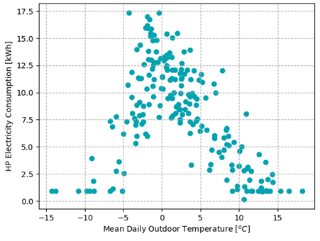
Figure 1. To ensure that the analysis period did not contain any days where the system was in cooling mode, the daily ASHP electricity consumption was plotted against the mean outdoor temperature. Cooling operation produces an upwards ASHP electricity consumption trend in warm conditions (which is not present in the example home here).
5.2 Step 1c: Determine Home Balance Point Temperatures
To estimate the home balance point temperatures for each home, the ASHP data was filtered and then fit with a regression line to find the x-intercept. The filtering excluded datapoints with a mean outdoor temperature above 16°C or below -5°C, and any datapoints with a furnace energy consumption above a threshold value. An example home is shown in Figure 2, where the building HBPT was estimated 14.3°C. HBPTs from all homes are shown in Table 6.
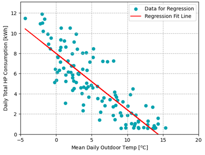
Figure 2. HBPTs (i.e. the outdoor temperature above which active heating is not required) was estimated from regression analysis of the ASHP electricity consumption data. In the example home shown in this plot, HBPT was estimated using the x-intercept at 14.3 oC.
Table 6. Estimated HBPTs for each home in the analysis
| Identifier | HBPT [oC] |
| H1 | 11.1 |
| H2 | 13.2 |
| H3 | 14.3 |
| H4* | 15.0 |
| H5 | 14.5 |
| H6 | 15.8 |
| H7 | 13.5 |
| H8 | 12.1 |
*H4 was estimated visually since the regression produced a poor value due to scatter in the data points.
5.3 Step 1d: Filter Data for Regression
Data was filtered to identify those points where the ASHP consumed no energy (or minimal energy, for example, due to standby loses). Filtering for an example home is shown in Figure 3. The datapoints used in the baseline furnace regression model are shown in blue – on these days the ASHP was not providing heat to the home (or the heat provided was negligible compared to the furnace) and heating was done by the furnace.
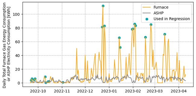
Figure 3. For the full heating season analysis period, furnace gas consumption (here shown in energy units of kWh) and ASHP electricity consumption were evaluated to identify days suitable to define a baseline furnace energy consumption model. Only those days where the ASHP was off (or had negligible electricity consumption) were considered.
5.4 Step 1e & 1f: Determine Regression Baseline Models
Regression analysis was used to define baseline furnace gas energy consumption models. These models predict the furnace gas energy consumption in the absence of the ASHP. The models estimate the daily furnace gas consumption as a function of the mean outdoor temperature. To define the model, data were filtered to include only those days where only the furnace was used to heat the home (Step 1d). The model was forced to go through the balance point identified in Step 1c. Results are shown in Figure 4. The coefficient of determination (R2) varies from 0.74 to 0.95.
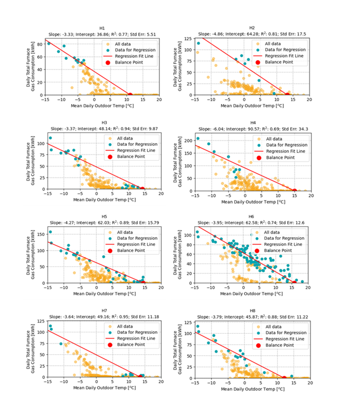
Figure 4. Baseline furnace energy consumption models were created for each home using data from those days where the ASHP energy consumption was negligible. Regression lines were forced to go through the HBPTs determined in a previous step because there was typically less data with furnace operation in warm temperatures.
6 Results: Gas Energy Savings
6.1 Steps 2a to 2d: Tabulate Actual Gas Consumption, Estimate Baseline, and Determine Gas Savings
The baseline furnace gas energy models were used to estimate the total baseline gas energy consumption for the analysis periods identified in Table 5 for each home. This was compared against the total actual gas consumption of the furnaces determined from the submeter data. Gas energy savings was determined as the difference between these two values. Modelled furnace gas energy baseline, actual furnace gas energy consumption, and calculated savings is shown in Figure 5. Error bars are from the uncertainty resulting from the regression modelling based on the standard error of the model and a 95% confidence interval.
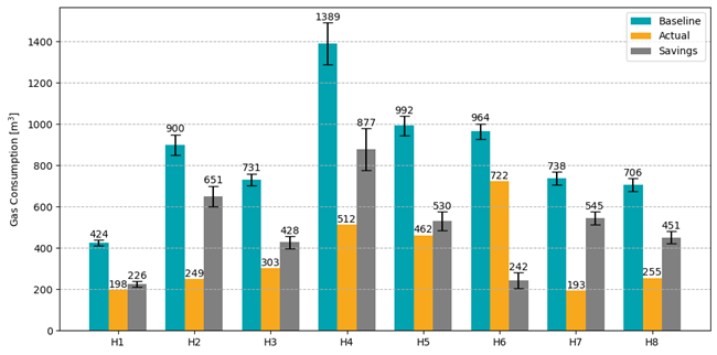
Figure 5. The modelled baseline gas consumption, actual gas consumption, and calculated savings are shown for each home in the study.
7 Results: ASHP Electricity Consumption in Heating Mode
7.1 Step 3a: Total ASHP Electricity Consumption
The total ASHP electricity consumption, corrected for any days omitted from the analysis, is shown in Figure 6.
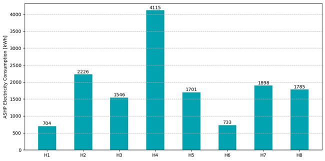
Figure 6. The ASHP electricity consumption is plotted for the full monitoring period of each home.
7.2 Step 3b & 3c: Controls Evaluation and TOU Breakdown
The effectiveness of the smart thermostats at achieving the intended control points (shown in Table 3) are evaluated in Figure 7 and Figure 8 as frequency histograms with respect to both outdoor temperature and TOU bracket. These plots are based on hourly-aggregated data and include the energy consumption data that is known to occur within a given hour. Effective economic balance points are shown as vertical lines in the corresponding TOU colour. The eEBPT for off-peak is shown as dashed green, that for mid-peak is solid yellow, and that for peak is dotted red. Figure 7 shows the ASHP electricity breakdown, and Figure 8 shows the furnace gas consumption breakdown. These plots cover the full heating season analysis period.
If the ASHP control is operating as expected, then the bars in Figure 7 should fall to the right of the EBPT shown in the corresponding colour. For example, red bars (indicating peak electricity consumption) should be seen to the right of the dotted red line but not to the left (or very minimally so). Note that there is some room for uncertainty due to small differences in the outdoor temperature data assumed by the thermostat and that used in this analysis. Overall, the ASHPs appear to be following the controls set-points.

Figure 7. The ASHP electricity consumption data was aggregated hourly and visualized as a frequency histogram incorporating both the outdoor temperature and the TOU. The control is operating as expected if the bars indicating energy consumption fall to the right of the eEBPT shown in the corresponding colour (i.e. the peak eEBPT is shown as the red dotted line and the red bars should be to the right of this line). The ASHP energy consumption profiles are overall near expectations across all homes. These plots cover the full heating season analysis period.
If the furnace control is operating as expected, then the bars in Figure 8 should fall to the left of the eEBPT shown in the corresponding colour. H1 and H7 are the best examples of the expected operation. However, to varying levels, the furnaces are sometimes used to provide heating when the ASHPs were predicted to be more economical. This is discussed further in the Discussion section. Note that it was worst for H6 because the thermostat was offline until January 2023, and this is also discussed further in the Discussion.
The breakdown of ASHP electricity consumption according to TOU is shown in Figure 9. The nature of the electricity monitoring (it was not logging data on a preset constant interval) was such that the consumption could sometimes not be placed in a TOU bracket. However, in every case, more than 79% of the data could be mapped to a TOU bracket. The breakdown was used to determine a weighted electricity rate. This is shown as the data label in units of cents per kWh.
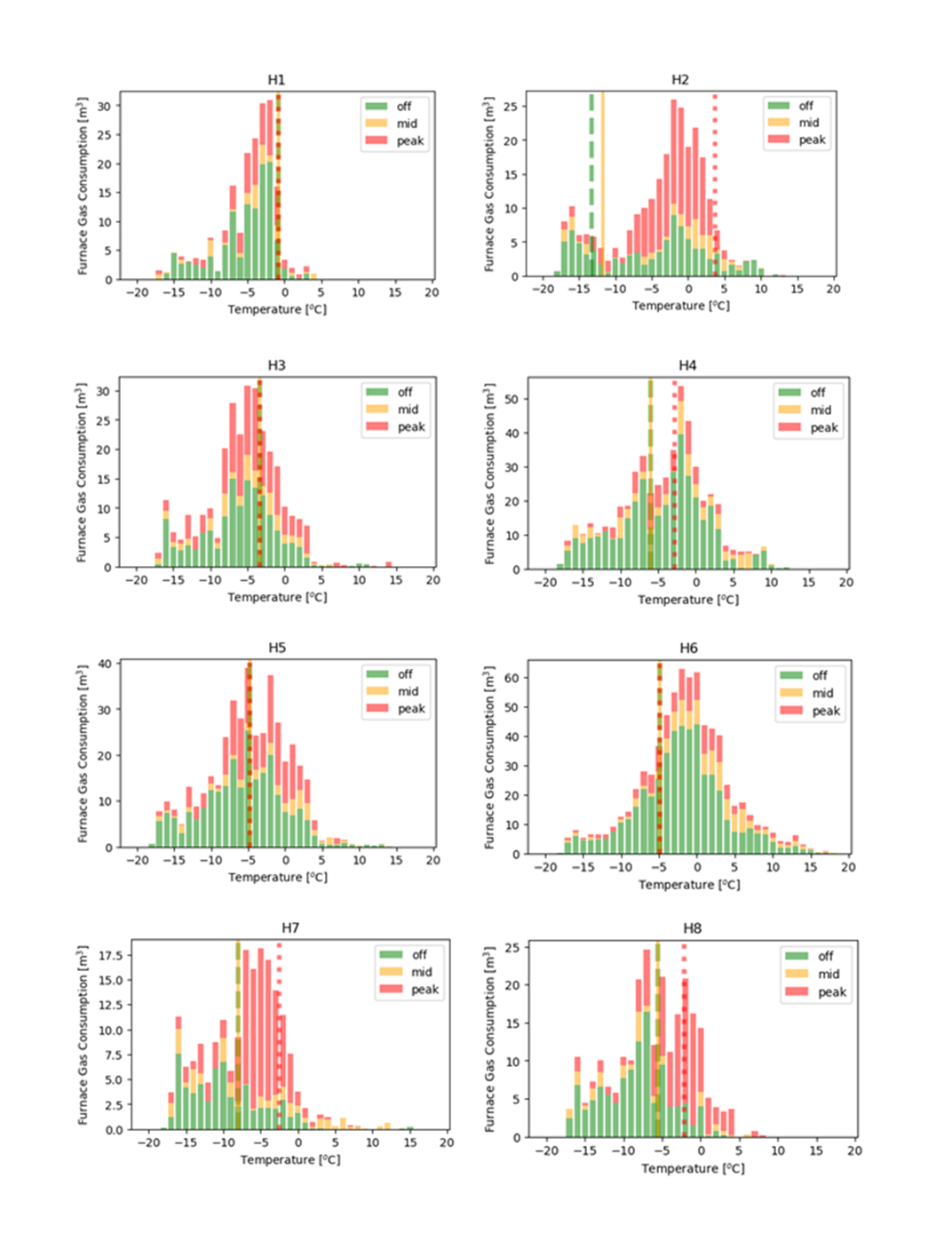
Figure 8. The furnace gas consumption was aggregated hourly according to TOU and outdoor temperature, and then visualized as a frequency histogram. The control is operating as expected if the bars indicating gas consumption fall to the left of the EBPT shown in the corresponding colour (i.e. the peak eEBPT is shown as the red dotted line and the red bars should be to the right of this line). To varying degrees, the furnaces are sometimes operating when the ASHP are predicted to be more economical. These plots cover the full heating season analysis period.
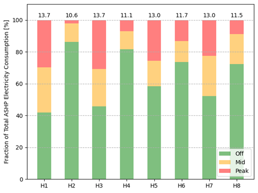
Figure 9. The electricity consumption of the ASHP was broken down according to TOU and then used to determine a weighted electricity rate (shown as the data label) in units of cents per kWh.
8 Results: Fraction of Heating from ASHP
8.1 Step 4a: Fraction of Heating
The fraction of heating space provided by the ASHP (versus the total heating provided by both ASHP and furnace) for the full heating season was calculated as the ratio of the gas savings over the modelled baseline. This is shown in Figure 10.
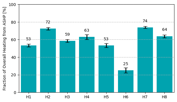
Figure 10. The fraction of heating provided by the ASHP was estimated for each home in the analysis. Uncertainty bars are due to the error of determining the baseline gas energy consumption using regression analysis.
9 Results: Estimated As-installed SCOP
9.1 Step 5a: SCOPs
The SCOPs were estimated as the gas savings (in energy units) multiplied by the furnace AFUE and divided by the ASHP electricity consumption. Results are shown in Figure 11.
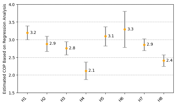
Figure 11. The estimated SCOPs from each ASHP are shown. Uncertainty bars are due to the error of determining the baseline gas energy consumption using regression analysis.
10 Results: Net Cost Savings
10.1 Step 6a to 6e: Net Heating Season Savings
A gas rate of 0.580 $/m3 was applied to the baseline furnace gas consumption to determine the baseline heating costs. Actual heating costs were determined by applying the weighted electricity rate determined for each home to the ASHP electricity consumption and adding that value to the cost of the gas that was actually consumed by the furnace. The net cost savings is the difference between baseline and actual.
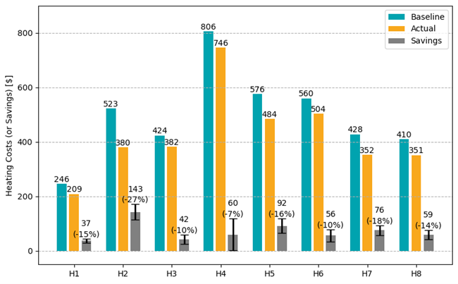
Figure 12. The baseline heating costs, actual heating costs, and estimated net savings from operating the ASHPs are shown. Uncertainty bars are due to the error of determining the baseline gas energy consumption using regression analysis.
10.2 Step 6f: Cooling Season Cost Reductions
Savings in cooling mode were assessed through direct comparison of the hourly whole-home utility data for Summer 2021 versus Summer 2022. In both years, June to August were considered. Assuming a balance point of 18oC, the total CDDs from Summer 2021 and Summer 2022 were within 2.5% of each other, with Summer 2022 being slightly lower. The pre- and post-retrofit periods therefore cover the same amount of time and the nearly same CDDs. Monthly electricity, highlighting the summer months, is shown in Figure 13.
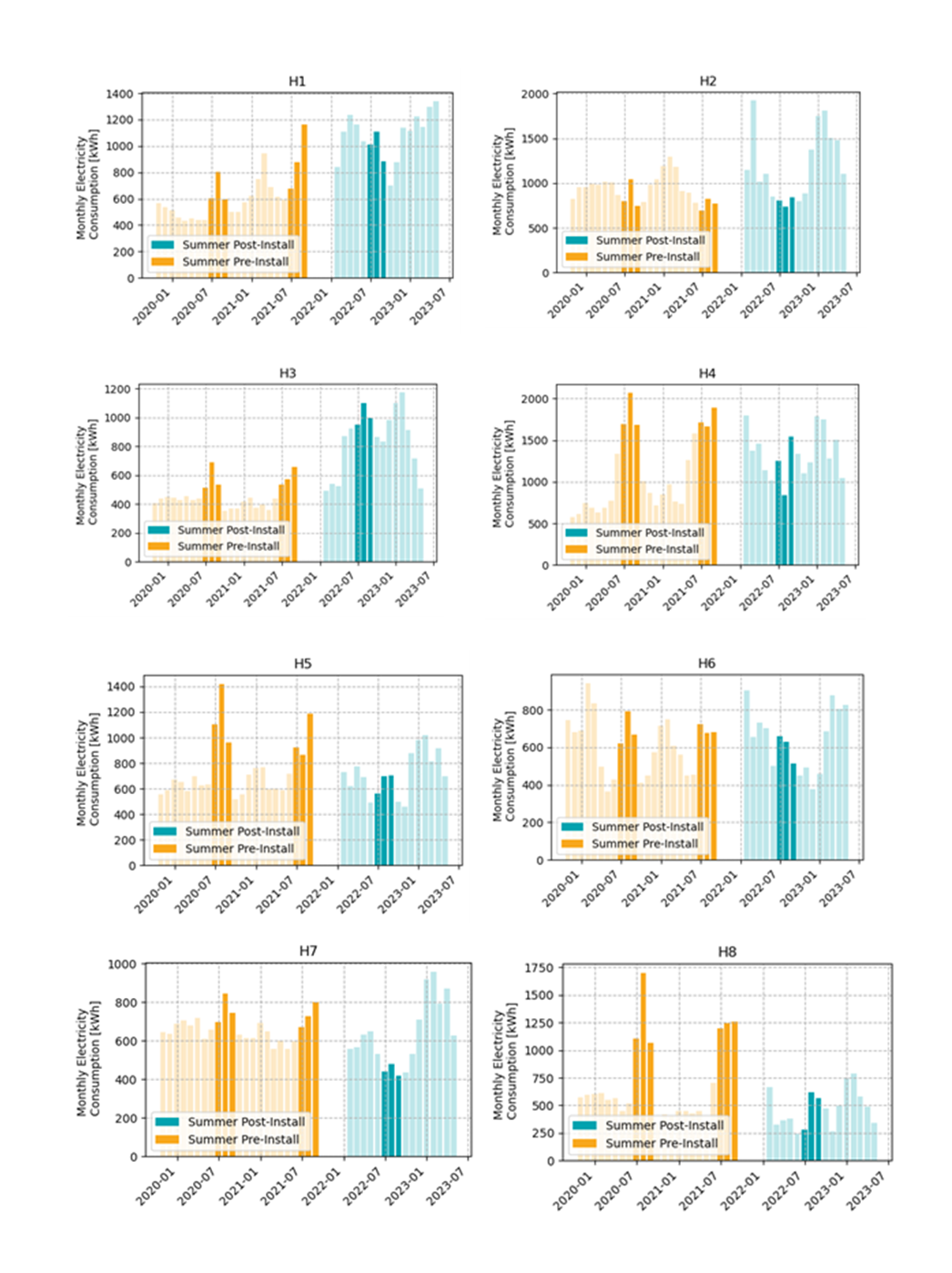
Figure 13. The pre- and post-retrofit monthly electricity consumption is shown for each home.
Homeowners were surveyed to identify any other energy-influencing factors impacting the home. The homeowner from H1 indicated that an additional occupant moved into the home for Summer 2022 that was not there Summer 2021. The homeowner from H3 indicated that an electrical device was added to the home for Summer 2022. It consumed on the scale of 500 W and was operated continuously. H8 did not respond to the survey. Homeowners did not flag other factors.
The daily electricity consumption of the homes for Summer 2021 and Summer 2022 are plotted in Figure 14 with respect to CDDs in order to identify any spurious data. Electricity consumption increases post-retrofit are apparent for H1 and H3, for the reasons discussed above. A drastic stepwise decrease occurred for H8, but it appears to be unrelated to the ASHP. Without having survey data for H8, it is not possible to determine the cause.
Stepwise changes were not observed for any other homes. However, behavioural changes like setpoint changes or actively turning off the A/C could still have impacted energy consumption. Overall, H1, H3, and H8 were not considered when estimating cooling mode savings based on their responses (or lack of response), and all other homes were considered. Savings are shown in Table 7. The average reduction in electricity bills between Summer 2021 and Summer 2022 was $94.
Table 7. Changes in whole-home summer electricity consumption pre- and post-retrofit.
| Summer 2021 kWh | Summer 2022 kWh | |||||||
| Identifier | Off | Mid | Peak | Off | Mid | Peak | Change in Consumption [kWh] | Cost Reduction [$] |
| H2 | 1,238 | 473 | 596 | 1,308 | 527 | 608 | -136 | -16 |
| H4 | 2,869 | 1,147 | 1,334 | 2,441 | 633 | 640 | 1,636 | 245 |
| H5 | 2,031 | 487 | 490 | 1,312 | 339 | 362 | 995 | 117 |
| H6 | 1,722 | 198 | 191 | 1,339 | 246 | 262 | 264 | 19 |
| H7 | 1,444 | 408 | 383 | 880 | 263 | 225 | 867 | 107 |
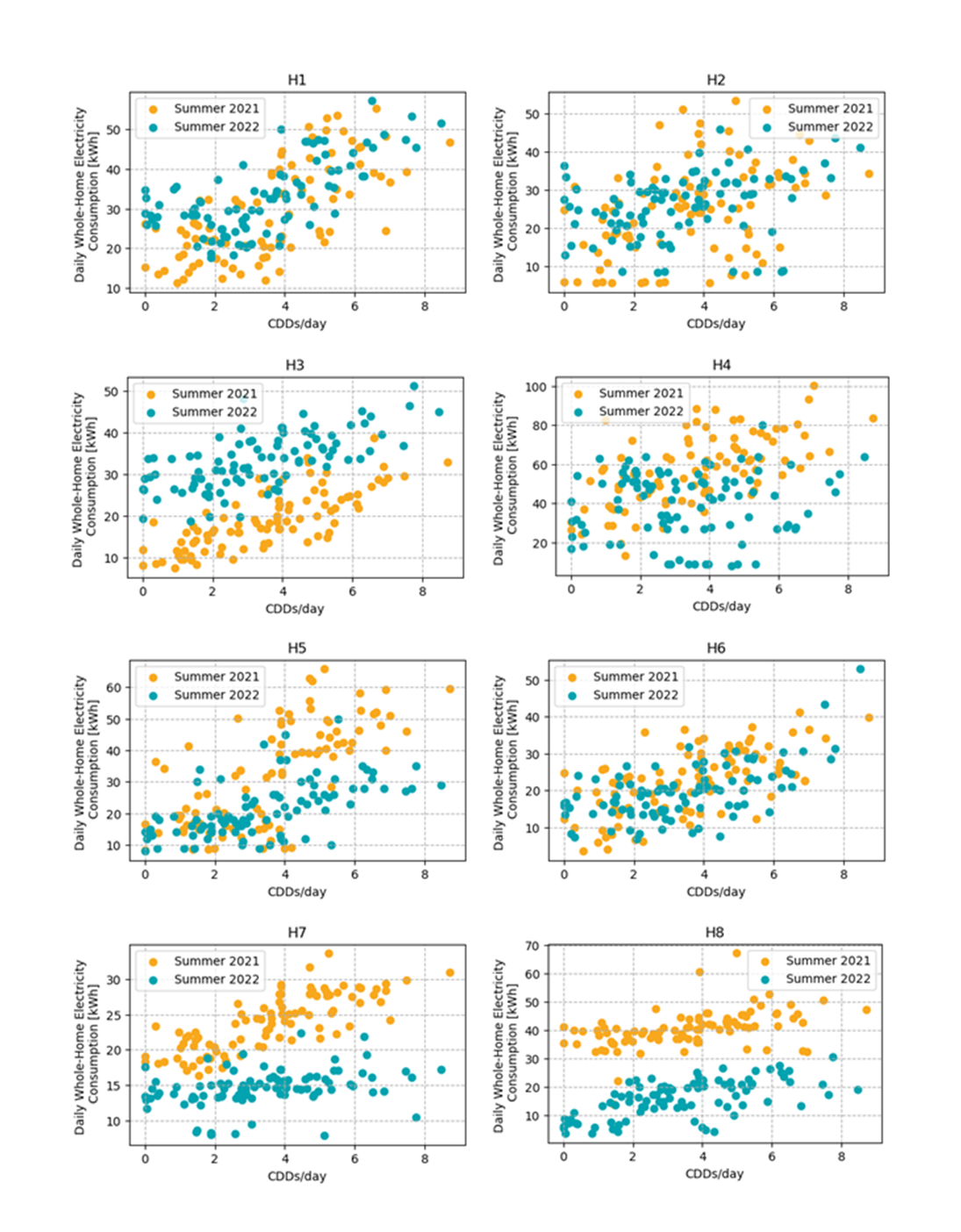
Figure 14. Daily whole-home electricity consumption was plotted as a function of CDDs for each home for both Summer 2021 and Summer 2022. Note that H1, H3, and H8, were not considered in the cooling savings calculation based on the survey responses.
10.3 Summary
A summary of the heating mode and cooling mode savings is provided in Table 8. It’s important to note that, due to the methodological differences in calculating savings, the heating mode savings are referenced to a new high-efficiency furnaces, whereas the cooling mode savings are in reference to the old A/C unit.
Table 8. Total savings summary
| Identifier | Heating Mode Savings [$] | Cooling Mode Savings [$] | Total Savings [$] |
| H1 | 37 | N/A | 37 |
| H2 | 143 | -16 | 127 |
| H3 | 42 | N/A | 42 |
| H4 | 60 | 245 | 305 |
| H5 | 92 | 117 | 209 |
| H6 | 56 | 19 | 75 |
| H7 | 76 | 107 | 183 |
| H8 | 59 | N/A | 59 |
| Average: | 71 | 94 | 130 |
11 Results: Electricity Demand Changes
11.1 Step 7a: Demand Changes
A comprehensive electricity demand analysis was outside of scope for this study. However, the hourly whole-home electricity consumption data provided by London Hydro offered a simple high-level look at how the electricity demand of the homes both individually and collectively pre- and post-retrofit. In this report, the term “demand” is intended to mean the maximum value that was reached for the hourly average power draw of the home.
For each home, the full hourly dataset that was provided was plotted (Figure 15). It encompassed Summer 2019 to Spring 2023. The analysis simply evaluated the difference between the peak demand of the house pre-retrofit and post-retrofit. Note that the study was not designed to be able to fully attribute these changes to the ASHPs and there may be other mitigating factors impacting demand.
In two cases, peak demand decreased post-retrofit. In six, it increased. The decreases were 12 to 15% and the increases were 6 to 25%. Often the peak demand is a pronounced increase that is limited to only a few hours of operation and not a value that regularly occurs.
The aggregated total demand across all 8 homes is shown in Figure 16. The maximum demand binned for each hour of the day is shown in Figure 17. The aggregated peak demand increased by 2% after the ASHPs were installed but this only occurred for 1 hour of operation post-retrofit. The remaining post-retrofit hours that were considered all had lower demand than the pre-retrofit peak demand.
Prior to the retrofits, the peak demand occurred during the cooling months. The cooling month peak was reduced after the retrofits. This is assumed to be due primarily to the increased efficiency of the new ASHPs versus the old existing A/C units. Post-retrofit, the new peak occurs during the heating months, but it is similar in scale to the pre-retrofit peak that occurred during the cooling months.
The demand impacts of individual homes were greater than the impacts on the aggregated demand of all homes because the demand peaks post-retrofit were typically limited to relatively few hours, and these hours did not align across all homes.
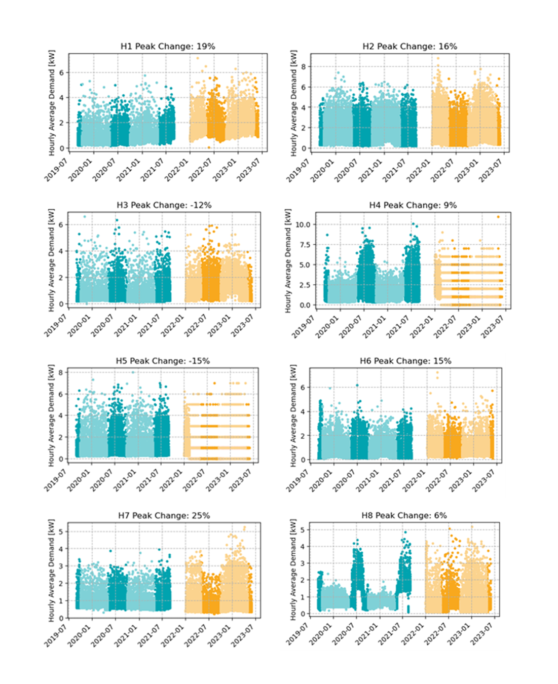
Figure 15. The hourly average electricity demand is plotted for all study homes. More than a year of data pre- and post-retrofit was considered. In two homes, peak demand decreased post-retrofit. In six homes, it increased. Some of the data for H4 and H5 looks strange post-retrofit because the data provided for analysis was rounded to the nearest integer for part of the post-retrofit period.
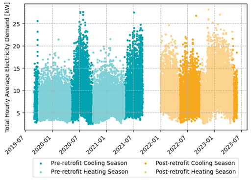
Figure 16. The hourly average electricity demand totaled across all 8 study homes is plotted as a time-series. More than a year of data pre- and post-retrofit is included. Post-retrofit, there is 1 hour that exceeds the pre-retrofit peak by 2%. All other hours post-retrofit are below the pre-retrofit peak.
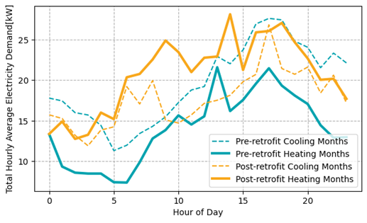
Figure 17. The demand data shown in Figure 16 was aggregated to determine the maximum power draw for each hour of the day, considering both the pre- and post-retrofit data. The demand during the cooling season generally decreased post-retrofit and the demand during the heating season increased.
12 Results: Net Carbon Reductions
12.1 Step 8a: Carbon Reductions
Carbon reductions depend on the emission factor for grid electricity. The grid is currently in a state of transition and different assumptions are possible for the grid EF. This is described in Section 4. The lower the EF for grid electricity, the better the net carbon reductions from using an ASHP. Baseline carbon emissions from the gas furnaces are shown in Figure 18. Heating season carbon emissions are shown as a percentage reduction in Figure 19 and in T CO2e Figure 20. Figure 21 shows the cooling season reductions and Figure 22, the total carbon emissions reductions.
Overall, with a relatively clean grid, the relative carbon reductions for home heating are large. However, in a worst-case scenario where the IESO 2022 projected MEFs are realized, the carbon emissions reductions in heating mode are low because the new electricity required for the ASHPs would largely be from natural gas plants. To be clear, this report does not claim that the IESO 2022 projected MEFs will be realized, especially considering upcoming new clean electricity regulations. Rather, it is only being evaluated as a scenario. It is clear that clean electricity is required to decarbonize homes with ASHPs.
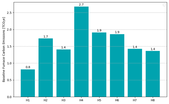
Figure 18. Baseline carbon emissions for space heating in each home by multiplying the baseline gas consumption with the gas emission factor.
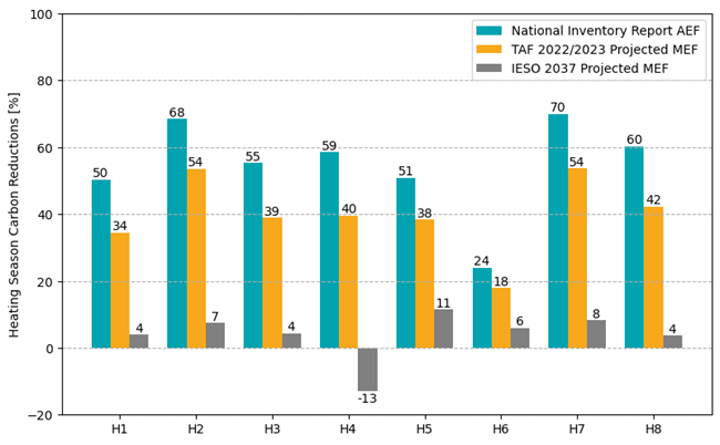
Figure 19. The relative carbon emission reductions for each home were calculated assuming different scenarios for the grid emissions factor (shown as different colours).
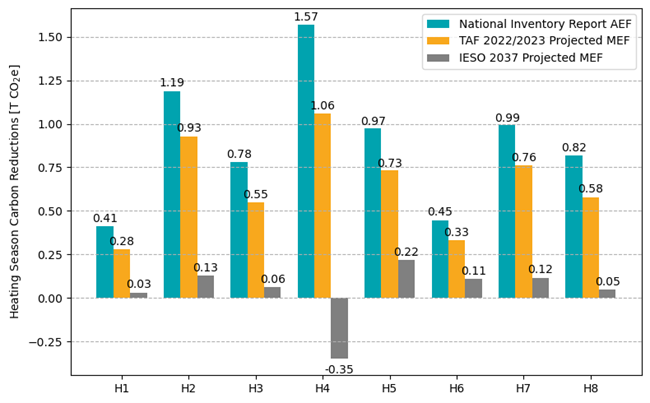
Figure 20. The carbon emission reductions in T CO2e for each home were calculated assuming different scenarios for the grid emissions factor (shown as different colours).
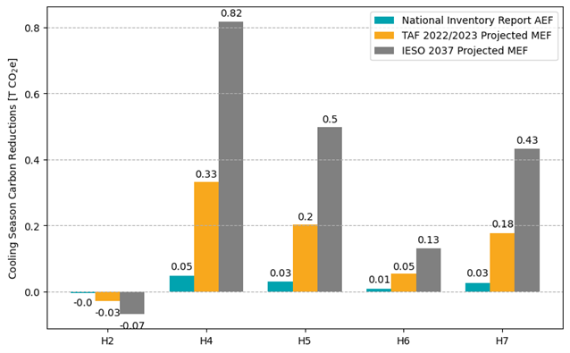
Figure 21. The cooling season carbon emissions are shown assuming different scenarios for the grid EF.
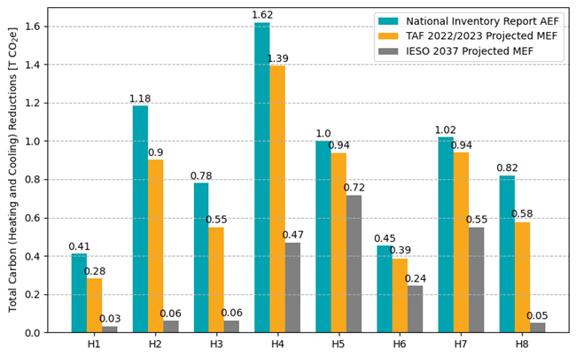
Figure 22. The total carbon emission reduction including both the heating and the cooling season are shown assuming different values for the grid EF.
13 Results: Summary
A summary of key metrics is provided in Table 9. A more detailed breakdown is provided in Table 10.
Table 9. High-level summary of key metrics
| Parameter | Unit | Minimum | Maximum | Average |
| Heating Mode Utility Savings | $ % | 37 7 | 143 27 | 71 15 |
| Cooling Season Utility Savings | $ | -16 | 245 | 94 |
| Heating Season Carbon Reductions (Based on Marginal Electricity Grid Emission Factor) | TCO2e % | 0.28 18 | 1.06 54 | 0.64 40 |
| Cooling Season Carbon Reductions | TCO2e | -0.03 | 0.33 | 0.15 |
| Fraction of Heating Provided by ASHP | % | 25* | 74 | 58* |
| Seasonal Coefficient of Performance | W/W | 2.1 | 3.3 | 2.8 |
| Annual Peak Demand Increase Post-retrofit | % | -15 | 25 | 2 |
*Only 25% of the heating was done by the ASHP in one home because of an issue that caused the ASHP to be off entirely for more than half the heating season. This home was an outlier. Not including this outlier, the minimum fraction of heating provided by the ASHP was 53%, and the average was 63%.
Table 10. Detailed summary of key parameters and metrics.
| Parameter | H1 | H2 | H3 | H4 | H5 | H6 | H7 | H8 |
| Furnace Capacity [kBTU/h] | 45 | 60 | 60 | 88 | 60 | 60 | 60 | 40 |
| ASHP Nominal Capacity [RT] | 2.5 | 3 | 2 | 3 | 1.5 | 1.5 | 2.5 | 3 |
| ASHP HSPF (Region IV) [BTU/h per W and (W per W)] | 9.5 (2.8) | 10 (2.9) | 9 (2.6) | 9.5 (2.8) | 9.5 (2.8) | 9.5 (2.8) | 9.5 (2.8) | 10 (2.9) |
| ASHP Compressor Type | Two-stage | Inverter | Two-stage | Two-stage | Single-stage | Single-stage | Single-stage | Inverter |
| Off-peak EBPT [oC] | -23.5 | -20.4 | -18.9 | -26.8 | -19.4 | -22.2 | -16.8 | -21.3 |
| Mid-peak EBPT [oC] | -16.2 | -11.7 | -13.4 | -18.1 | -14.2 | -17.7 | -11.6 | -12.8 |
| Peak EBPT [oC] | -3.2 | 3.7 | -3.9 | -2.8 | -5 | -9.9 | -2.5 | 2.1 |
| TBPT [oC] | -0.8 | -13.3 | -3.3 | -6.0 | -4.8 | -4.9 | -8.0 | -5.6 |
| Off-peak eEBPT [oC] | -0.8 | -13.3 | -3.3 | -6.0 | -4.8 | -4.9 | -8.0 | -5.6 |
| Mid-peak eEBPT [oC] | -0.8 | -11.7 | -3.3 | -6.0 | -4.8 | -4.9 | -8.0 | -5.6 |
| Peak eEBPT [oC] | -0.8 | 3.7 | -3.3 | -2.8 | -4.8 | -4.9 | -2.5 | 2.1 |
| Baseline Furnace Gas Consumption [m3] | 424 | 900 | 731 | 1,389 | 992 | 964 | 738 | 706 |
| Actual Furnace Gas Consumption [m3] | 198 | 249 | 303 | 512 | 462 | 722 | 193 | 255 |
| Gas Savings [m3] | 226 | 651 | 428 | 877 | 530 | 242 | 545 | 451 |
| Fraction of Total Heating Provided by ASHP [%] | 53 | 72 | 59 | 63 | 53 | 25 | 74 | 64 |
| Total ASHP Electricity Consumption (Heating Season) | 755 | 2,226 | 1,546 | 4,115 | 1,701 | 733 | 1,898 | 1,785 |
| ASHP Electricity Consumption TOU Breakdown (Off/Mid/Peak) [%] | 42/28/30 | 86/12/2 | 46/23/31 | 82/11/7 | 58/16/26 | 74/13/13 | 52/25/23 | 72/19/9 |
| Total Cooling Season Electricity Reduction [kWh] | N/A | -136 | N/A | 1,636 | 995 | 264 | 867 | N/A |
| As-installed SCOP [W per W] | 3.2 | 2.9 | 2.8 | 2.1 | 3.1 | 3.3 | 2.9 | 2.4 |
| Heating Season Cost Savings [$] | 37 | 143 | 42 | 60 | 92 | 56 | 76 | 59 |
| Cooling Season Cost Savings [$] | N/A | -16 | N/A | 245 | 117 | 19 | 107 | N/A |
| Total Cost Savings [$] | 37 | 127 | 42 | 305 | 209 | 75 | 183 | 59 |
| Heating Season Carbon Reductions [TCO2e and (%)] | 0.28 (34) | 0.93 (54) | 0.55 (39) | 1.06 (40) | 0.73 (38) | 0.33 (18) | 0.76 (54) | 0.58 (42) |
| Cooling Season Carbon Reductions [TCO2e] | N/A | -0.03 | N/A | 0.33 | 0.20 | 0.05 | 0.18 | N/A |
| Total Carbon Reductions [T CO2e] | 0.28 | 0.90 | 0.55 | 1.39 | 0.94 | 0.39 | 0.94 | 0.58 |
| Change in Peak Electricity Demand [%] | 19 | 16 | -12 | 9 | -15 | 15 | 25 | 6 |
14 Discussion
14.1 ASHP Sizing
From Section 2, it was clear that the sizing of some ASHPs reduced the potential for savings. In 4 cases, the thermal balance point was higher than the economic balance points and the ASHPs were not large enough to optimize savings through smart-switching. Since these homes were operating on conventional single-point temperature switchover (where the eEBPT was the same across all TOUs), smart-switching did not offer any benefits over conventional single-point temperature switchover control.
Larger ASHPs or ASHPs with better cold-temperature capacity maintenance (or both) would offer greater net cost savings and carbon reductions as well as better potential for optimization through smart switching control. However, ASHP size needs to be carefully considered such that the system will work within the constraints of the home (for example, with the existing ductwork or electrical panel). It may also be possible to find solutions that will allow larger ASHP sizing within these constraints.[16]
As mentioned previously, the NRCan ASHP Sizing and Selection Toolkit[2] can help contractors to estimate key parameters like the economic and thermal balance points, the fraction of heating that will be done by the ASHP, and the expected cost of operation. This is helpful information to achieve a right-sized ASHP for homeowners based on their needs. Overall, additional contractor training is needed.
14.2 Home Size
The baseline gas consumption shown in Figure 5 indicates that homes considered in this study are primarily small-to-medium sized homes. Enbridge noted that the estimated furnace gas consumption for an average customer’s home is larger than was seen in this study. Note that cost savings scales with home size and heat load, and greater cost savings are expected for homes that consume larger amounts of gas for heating.
14.3 Weather
The winter of 2022-2023 was warm compared to the recent past. Total heating season HDDs for the past 10-years are shown in Figure 23. Winter 2022/2023 had approximately 10% fewer HDDs than the mean value for the past 10-years.
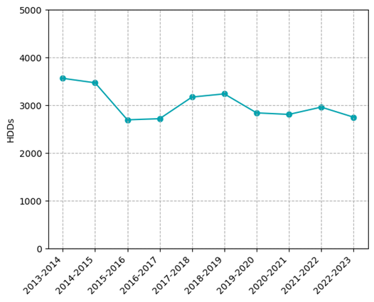
Figure 23. The HDDs from Sept 15th to April 15th for the past 10 years were summed. Winter 2022/2023 is approximately 10% lower than the historical mean.
Note that the impacts of warmer weather are not straightforward. On one hand, greater ASHP efficiency might be expected in warmer conditions but on the other hand, there are fewer heating hours from which to generate savings. The impacts of weather were not evaluated. It is possible to apply the baseline furnace consumption models to weather from different years, but the energy consumption of the ASHP and furnace were not modelled and therefore could not be easily applied to different weather datasets.
14.4 Sensitivity to Utility Rates
This analysis determined the savings for approximately one year in 2022/2023. The systems are expected to last on the scale of 15 years. Future utility rates are subject to change. For example, the Federal Carbon Charge schedule indicates that it will add an additional 22.61 cents/m3 (+HST) to the cost of gas by 2030.[17] Note that the Climate Action Incentive provides back to taxpayers the proceeds of this charge. Overall, the future rates can’t be predicted with accuracy. The savings will change as the rates change but evaluating the impact of changing utility rates on savings would involve a more complicated theoretical modelling exercise that was beyond the scope of this study. From an operating cost perspective, a benefit of the smart-switching controller is that it is always predicted to produce some level of savings as it reconfigures its setpoints to adjust for changing rates.
14.5 Factors for Optimizing Cost Savings
H2 had the largest savings, and it is useful to look at the key factors impacting these savings. H2 had a high-efficiency ASHP that could a handle a large fraction of the annual heating load and it selectively curtailed any operation during a peak TOU using smart control such that it was almost always being powered by lower cost electricity. Moreso than any other home, H2 best showcases the economic and carbon savings potential for smart control.
14.6 COP Variation
There are different reasons why the as-installed estimated SCOP may vary from the expected value based on the AHRI-rated HSPF. Weather is an important factor. The HSPF is intended to be a weather-averaged efficiency value. HSPF is in units BTU/hr per Watt but can similarly be expressed as Watt/Watt (the familiar COP unit) by dividing by a factor of 3.41. For example, an HSPF 9.0 translates to an SCOP of 2.6.
HSPF[18] values are typically provided for Region IV and this covers much of the U.S. Much of Canada is covered by Region V (which is colder), but in reality, Southern Ontario’s climate lies somewhere in between Region IV and Region V. It follows that the actual SCOP for a Southern Ontario installation may be less (on average) than the SCOP derived from the Region IV HSPF simply because the weather is colder than Region IV.
Hybrid installations may also achieve higher SCOPs when they are selectively being controlled to operate in warmer weather. The rated HSPF is weighted down by assuming that the ASHP operates in cold conditions. If the ASHP in an actual installation only operates in milder conditions, then the real-world SCOP may be higher than the SCOP implied by the rated HSPF.
As-installed factors may influence the real-world SCOP as well. Key factors include (i) compressor cycle times, (ii) thermostat setpoint temperatures, (iii) airflows, (iv) defrost control algorithms, and (v) whether the system was installed and commissioned correctly. If a single-stage or two-staged ASHP is rapidly cycling on and off, then it would degrade SCOP. SCOP is also degraded for higher return temperatures. Standardized testing assumes 21.1 oC but some homeowners may prefer warmer temperatures in their own home. If the needed airflow is not achieved, (for example, the ductwork is constrained, or the furnace dip switches are not configured properly) the real-world SCOP may be lower as well.
In this study, data was not collected on return temperatures or airflow, and the electrical submetering was too coarse to characterize the cycling behaviour. A full explanation behind the variation in SCOP is therefore not possible.
14.7 Smart Control and Furnace Operation
Figure 7 and Figure 8 showed that the ASHP generally followed the expected control setpoints, but the furnace sometimes did not follow the control set-points (to varying degrees in each home). H6 was the most obvious case.
The thermostat manufacturer explained that the H6 homeowner’s thermostat was offline from October 8, 2022, until January 12, 2023. The initial disconnect resulted from a firmware upgrade. The homeowner did not respond to the initial email that was sent offering to reconnect after the upgrade (sent on October 11th), but they eventually reached out to the thermostat manufacturer in January and were reconnected.
In other cases, discussions with the thermostat manufacturer indicated that the ASHP may be overridden, with the system reverting to the furnace, when Emergency Heat Mode is manually selected. The system also reverts to the furnace when the thermostat does not have an internet connection.
It follows that the furnaces are operating more frequently than expected in some homes due to (i) manual changes to the thermostat mode from the homeowner, (ii) internet connectivity issues, and/or (iii) a disconnection event from a firmware upgrade.
Greater savings are likely if thermostat manufacturers are able to reduce the extent to which the systems default to the furnace unnecessarily. For example, local outdoor air temperature sensors might be used to reduce the dependence on the internet for temperature readings. Furthermore, the default operation without web connectivity may instead be to always attempt the ASHP first and then revert to the furnace if the ASHP is unable to meet the setpoint within a given timeframe.
14.8 Approach to Determining ASHP Efficiency and Savings
The use of regression analysis to estimate energy savings is the standard protocol in large buildings. However, many residential ASHP monitoring pilots tend to focus on directly measuring the COP through high-resolution instantaneous measurements of power consumption, supply and return temperatures, airflow, as well as (ideally) humidity and barometric pressure.
The challenge of the instantaneous COP-monitoring approach is that airflows and air temperatures may vary greatly across the cross section of the heat pump supply. Properly calibrated integrating grids (both for temperature and airflow) are normally required for accurate independent measurements. These grids sample airflow or temperature across many points of the duct cross-section to ensure that the recorded value accurately captures this variation. In a residential setting this can be prohibitively challenging, costly, and prone to error. Furthermore, this approach puts COP first and from that may deduce the energy/cost savings later – but energy/cost savings are often the most relevant parameters to a homeowner.
Conversely, the approach used in this analysis determines energy savings first, and then deduces the average SCOP based on the gas savings, electricity increase, and furnace efficiency. It’s important to note that if the SCOP can be used to estimate the energy savings, then it is just as valid to use the energy savings to determine the SCOP.
The benefit of this approach is that metering energy consumption is generally more straightforward and less costly than measuring parameters like airflow. It is also frequently possible to take this approach without any specialized data monitoring, utilizing only the available utility bills and qualitative information provided by the homeowner.
In the regression analysis approach, uncertainty comes from the quality of the baseline regression models. However, the gas consumption of a home is typically highly linear (because the heat loss equation is linear) and well represented by a linear regression model. Furthermore, the math for propagating the uncertainty of the model to other calculated parameters is well-defined.
Overall, the regression analysis approach is a lower-cost and accurate approach for residential heat pump performance analysis when compared to more costly and invasive approaches using instantaneous COP-monitoring. In an ideal study, both approaches would be undertaken and arrive at similar values, but this is often not feasible.
14.9 Optimizing Carbon
The smart-switching thermostats were configured to optimize operating cost reductions. However, it is worth noting that for temperatures that are slightly below the EBPTs, the ASHP is only slightly more costly to operate. It would be helpful for homeowners if smart-switching thermostats were equipped with a mode of operation that considered both cost and carbon savings optimization, rather than just “cost-only”. The thermostats in this study had this function but the pilot focused on cost benefits, and homeowners did not use the carbon optimization feature.
It may be the case that notable increases in carbon reductions are achievable for very small increases in operating cost when compared to a “cost-only” optimization approach. Carbon emission reductions may be increased further if the IESO released real-time marginal emission factor data which smart thermostats could then consider within their algorithms.
14.10 Notable Study Limitations
Study limitations are summarized below.
- The study focused on performance analysis of the pilot systems using submetering data and utility data. The study design was not able to offer a direct comparison of all-electric ASHPs, hybrid ASHPs with conventional controls, and smart-switching hybrid ASHPs; nor was a theoretical comparison offered.
- Heating mode savings are referenced to the furnace operating with the heat pump. The homeowner will have had greater savings if the furnace AFUE was upgraded alongside the ASHP installation but this additional potential savings from an upgraded furnace AFUE was not considered.
- Cooling mode savings are referenced to the A/C unit that was installed previously (which were older lower efficiency models) and not against a new high-SEER A/C unit. This was a limitation of the study design, which focused on the actual data submetering, and utility data collected from the installations.
- Qualitative analysis on the homeowner experience, the contractor experience, or the overall business case for the systems was outside of scope.
- Switching points were selected by the thermostat manufacturer, and the authors did not review the calculation process or determine if these are indeed the optimal values based on the real-world data that was collected.
- Based on the furnace energy consumption models, the homes are small-to-medium in size. Greater savings are possible in homes that consume more gas.
- This study only considered data for Winter 2022/2023 and did not extrapolate results to estimate performance in other years. Winter 2022/2023 was warmer than the historical average. While this may produce a higher SCOP, overall savings may be reduced when compared to a year that was closer to the historical average.
- Blower current consumption was collected and analyzed, but it was deemed a small enough factor that it was not considered in the main body of this report.
- The SCOP calculation assumed that the rated AFUEs of the furnaces were achieved in practice.
- The electricity meter used to determine the ASHP electrical consumption was not provided with an accuracy specification from the manufacturer, and any uncertainty resulting from the sensor was not included in the error bars that were estimated.
- The survey responses showed that three of the homes had fireplaces (H4, H5, and H7), three did not (H1, H2, and H6), and two did not specify if there was a fireplace in the home. Of those that had fireplaces, H4 specified the usage was light, H5 specified daily usage, and H7 specified that usage of the fireplace was rare. The fireplace gas consumption was not submetered. For H5, and potentially also H4, the usage of the fireplace could have impacted the analysis if it was proportionally greater (or lower) on those days used to create the baseline gas consumption model. Since the gas consumption model was created based on days where the outdoor temperature was colder, the likelier scenario is that fireplace consumption may have proportionally higher for those used to create the baseline furnace gas consumption model and the model may therefore underpredict baseline furnace gas consumption for the rest of the heating season. If the baseline gas model underpredicts gas consumption of the furnace, then the ASHP performance metrics would appear to be poorer (lower COP, lower fraction of heating, etc.). H4 had the lowest estimated SCOP in this study at 2.1. Disproportionately higher usage of the fireplace on colder days may offer a partial explanation.
- As of 2023, ultra-low overnight (ULO) electricity rate structures are now available in some Ontario jurisdictions, including London. It is generally expected that this would further reduce system heating costs when using a smart-switching hybrid system because the system could selectively operate the ASHP in the ultra-low and off-peak TOU brackets while avoiding ASHP operation in the new peak bracket. However, homeowners would have to evaluate for themselves whether the new ULO bracket would reduce energy costs for the full home. The new ULO rate structure could not be evaluated in this work.
14.11 Recommendations for Future Work
A recommendation for future work is that more research on the demand impacts of electrifying home heating loads with hybrid systems is needed. In this study, the home heating loads were 58% electrified on average and the aggregated annual peak electricity demand of the homes increased by only 2%.
It would be helpful for broadscale planning to better understand (based on real-world data) how peak demand is impacted by hybrid systems on a broadscale and how factors like the ASHP efficiency, ASHP sizing, and control algorithm influence peak demand.
From a demand perspective, it is also prudent that smart thermostats be equipped with the ability to participate in future utility demand side management programs that may seek to actively curtail ASHP electricity consumption during times of grid congestion. Active demand management may help to overall increase the total penetration of ASHPs on the grid while mitigating potential negative grid impacts.
In the context of decarbonization of homes through electrification, recent work theoretical modelling analysis has evaluated the demand peak mitigation benefits of different technologies including distributed electric and thermal storage as well as geothermal[19]. Future work should also consider how hybrid heating may compliment these other technologies.
14.12 Opportunities to Increase Cost and Carbon Reductions
Overall, three key areas of potential improvements for both operating cost and carbon emissions reductions were identified.
1.Avoiding unnecessary defaulting to the furnace: Thermostat manufacturers should explore ways to avoid unnecessarily defaulting to the furnace, specifically when there is a web-connectivity issue.
2.Improving ASHP sizing and selection to achieve more optimal savings: If the goal is to maximize operational cost and carbon savings, ASHPs should be sized to cover as much of the heating load as possible within the constraints of the home and budget. Contractor training is needed to help ensure optimal system sizing moving forward, and that the appropriate sizing and selection tools are effectively used.
3.Considering carbon reductions in the thermostat control algorithm: It would be helpful for homeowners if smart-switching thermostats were equipped with a user-selectable mode of operation that considered both cost and carbon savings optimization. It would be further beneficial if marginal emissions factor data were published in real-time from the IESO, such that this could be an input to future thermostat algorithms.
15 Conclusion
This report provided performance analysis results from eight homes participating in the smart hybrid heating pilot conducted in London, ON, by Enbridge Gas Inc. and London Hydro. The data analysis showed that the ASHPs used in the smart-switching hybrid systems:
- reduced the utility costs of the home,
- provided most of the home heating needs,
- reduced carbon emissions,
- operated with a high-efficiency, and
- did not significantly increase the aggregated peak electricity demand of the homes.
Moving forward, it is suggested that thermostat manufacturers seek to avoid unnecessarily defaulting to the furnace, and also that they additionally consider carbon reductions within their control algorithms. It is also suggested that contractor training is needed to help ensure optimal system sizing, and that the appropriate sizing and selection tools are effectively used.
Overall, this study builds confidence in ASHP technology generally. It provides further data and analysis to show that they are indeed high-performance devices that can reduce carbon emissions and homeowner utility costs.
16 References and Endnotes
[1] Note that it is not claimed that this study is IPMVP-adherent. Adherence to IPMVP would have required additional components like the creation of a formal IPMVP-adherent M&V Plan. The methodology was informed by the IPMVP only, and strict adherence is not claimed.
[2] NRCan ASHP Sizing and Selection Toolkit: https://natural-resources.canada.ca/maps-tools-and-publications/tools/modelling-tools/toolkit-for-air-source-heat-pump-sizing-and-selection/23558
[3] https://www.monnit.com/products/sensors/pulse-counter/single-input/
[4] The exact monitoring periods from Winter 2022/2023 for each home are provided in Section 5.1.
[5] https://london.weatherstats.ca/
[6] The outdoor temperature above which active heating is no longer required by the home.
[7] This was forced because typically there was colder temperature furnace consumption data to define the model, but more limited warm temperature data.
[8] Gas savings (in energy units) multiplied by the AFUE is an estimate of the total heat energy that was delivered by the ASHP.
[9] https://www.oeb.ca/sites/default/files/qram-egi-union-20221001-en.pdf and https://www.oeb.ca/sites/default/files/qram-union-20230101-en.pdf
[10] https://www.oeb.ca/consumer-information-and-protection/bill-calculator
[11] National Inventory Report 1990-2021: Greenhouse Gas Sources and Sinks in Canada, Part 2, Table A6.1-1 and Table A6.1-3. Emission factors from CO2, CH4, and N2O were combined.
[12] National Inventory Report 1990-2021: Greenhouse Gas Sources and Sinks in Canada, Part 3, Table A13-7.
[13] Available here: https://taf.ca/publications/electricity_emissions_factors/
[14] Available here: https://www.ieso.ca/en/Sector-Participants/Planning-and-Forecasting/Annual-Planning-Outlook
[15] More information here: https://www.canada.ca/en/services/environment/weather/climatechange/climate-plan/clean-electricity-regulation.html
[16] For example, options for home heating electrification without an electrical service upgrade are discussed in a report from Passive House Alberta released October 2023 titled “Electrification of Homes Without an Electrical Service Upgrade.” The report points to options like load management technology or opportunities to reduce other loads on the electrical panel.
[17] Impacts of Federal Carbon Charge on gas rates is explained on the Enbridge webpage here: https://www.enbridgegas.com/en/residential/my-account/rates/federal-carbon-charge#:~:text=What%20is%20the%20federal%20carbon,cubic%20metre%20(m3)
[18] Note that HSPF is currently being phased out and replaced by HSPF2.
[19] McDiarmid, Heather. An Analysis of the Impacts of All-Electric Heat Pumps and Peak Mitigation Technologies on Peak Power Demand in Ontario. Prepared for the Ontario Clean Air Alliance. November 15th, 2023. https://www.cleanairalliance.org/an-analysis-of-the-impacts-of-all-electric-heat-pumps-and-peak-mitigation-technologies/
17 STEP
The Sustainable Technologies Evaluation Program (STEP) is a multi-agency initiative developed to support broader implementation of sustainable technologies and practices within a Canadian context. STEP works to achieve this overarching objective by:
- Carrying out research, monitoring and evaluation of clean water and low carbon technologies;
- Assessing technology implementation barriers and opportunities;
- Developing supporting tools, guidelines, and policies;
- Delivering education and training programs;
- Advocating for effective sustainable technologies; and
- Collaborating with academic and industry partners through our Living Labs and other initiatives.
Technologies evaluated under STEP are not limited to physical devices or products; they may also include preventative measures, implementation protocols, alternative urban site designs, and other innovative practices that help create more sustainable and livable communities.
18 Notice
The contents of this report do not necessarily represent the policies of the supporting agencies. Although every reasonable effort has been made to ensure the integrity of the report, the supporting agencies do not make any warranty or representation, expressed or implied, with respect to the accuracy or completeness of the information contained herein. Mention of trade names or commercial products does not constitute endorsement or recommendation of products or services.
19 Acronyms
- AFUE: annual fuel utilization efficiency
- ASHP: air-source heat pump
- BTU: British thermal unit
- COP: coefficient of performance
- eEBPT: effective economic balance point temperature
- EBPT: economic balance point temperature
- HBPT: home balance point temperature
- HDD: heating degree day
- HSPF: heating season performance factor
- IPMVP: International Performance Measurement and Verification Protocol
- M&V: measurement and verification
- SCOP: seasonal coefficient of performance
- TOU: time-of-use
- TBPT: thermal balance point temperature
- RT: refrigeration ton
20 Acknowledgements
STEP gratefully acknowledges funding support for this study provided by The Atmospheric Fund (TAF). Base funding for STEP is provided by the City of Toronto, Region of Peel, and York Region. STEP also acknowledges in-kind support for personnel time (for tasks such as data collection, data sharing, and review) from both London Hydro and Enbridge Gas Inc. Note that Enbridge Gas Inc. did not provide financial contributions to STEP to perform this study.